
Journal of Geographical Sciences >
Urbanization, economic growth, and carbon dioxide emissions in China: A panel cointegration and causality analysis
Author: Liu Yansui (1965-), Professor, specialized in land sciences, sustainable agriculture and rural development. E-mail: liuys@igsnrr.ac.cn
*Corresponding author: Zhou Yang (1984-), PhD and Assistant Professor, E-mail: zhouyang@igsnrr.ac.cn
Received date: 2015-08-20
Accepted date: 2015-09-30
Online published: 2016-02-25
Supported by
National Natural Science Foundation of China, No.41130748, No.41471143
Major Program of National Social Science Foundation of China, No.15ZDA021
Copyright
Elucidating the complex mechanism between urbanization, economic growth, carbon dioxide emissions is fundamental necessary to inform effective strategies on energy saving and emission reduction in China. Based on a balanced panel data of 31 provinces in China over the period 1997-2010, this study empirically examines the relationships among urbanization, economic growth and carbon dioxide (CO2) emissions at the national and regional levels using panel cointegration and vector error correction model and Granger causality tests. Results showed that urbanization, economic growth and CO2 emissions are integrated of order one. Urbanization contributes to economic growth, both of which increase CO2 emissions in China and its eastern, central and western regions. The impact of urbanization on CO2 emissions in the western region was larger than that in the eastern and central regions. But economic growth had a larger impact on CO2 emissions in the eastern region than that in the central and western regions. Panel causality analysis revealed a bidirectional long-run causal relationship among urbanization, economic growth and CO2 emissions, indicating that in the long run, urbanization does have a causal effect on economic growth in China, both of which have causal effect on CO2 emissions. At the regional level, we also found a bidirectional long-run causality between land urbanization and economic growth in eastern and central China. These results demonstrated that it might be difficult for China to pursue carbon emissions reduction policy and to control urban expansion without impeding economic growth in the long run. In the short-run, we observed a unidirectional causation running from land urbanization to CO2 emissions and from economic growth to CO2 emissions in the eastern and central regions. Further investigations revealed an inverted N-shaped relationship between CO2 emissions and economic growth in China, not supporting the environmental Kuznets curve (EKC) hypothesis. Our empirical findings have an important reference value for policy-makers in formulating effective energy saving and emission reduction strategies for China.
Key words: urbanization; economic growth; CO2 emissions; panel cointegration; Granger causality
LIU Yansui , YAN Bin , *ZHOU Yang . Urbanization, economic growth, and carbon dioxide emissions in China: A panel cointegration and causality analysis[J]. Journal of Geographical Sciences, 2016 , 26(2) : 131 -152 . DOI: 10.1007/s11442-016-1259-2
Table 1 Data description and sources |
| Indicators | Unit | Abbreviation | Meaning of indicators | Sources |
|---|---|---|---|---|
| Built-up area | km2 | BA | Land urbanization | CCSY |
| Urban population | persons | UP | Demographic urbanization | CSY |
| GDP per capita | yuan RMB | pGDP | Economic growth | CSY |
| CO2 emissions | million tons | CO2 | Pollutant emissions | Guan et al., 2012 |

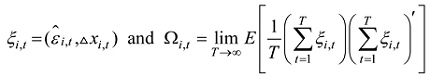 is the long-run covariance for this vector process which can be decomposed into
 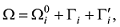 where
where  is the contemporaneous covariance and
  is a weighted sum of auto-covariance.
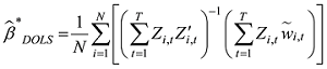
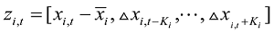 is vector of regressors, and
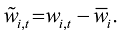
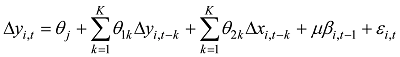
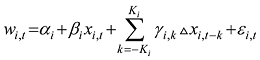
 is the error correction term with lag 1; εi,t is the residuals of the mode; μ is the coefficient of the error correction term βi,t-1. The significance of causality results is determined by Wald F-test. In the short-run, the x does not Granger cause y where H0: θ2k=0 for all i and k, while the long-run causality can be established if μ=0.
 Under the alternative hypothesis, there exists a causal relationship from x to y for at least one province of the sample. The test statistic is given by the cross-sectional average of individual Wald statistics defined for the Granger non-causality hypothesis for each province:
 for fixed T samples is as follows (Dumitrescu and Hurlin (2002):

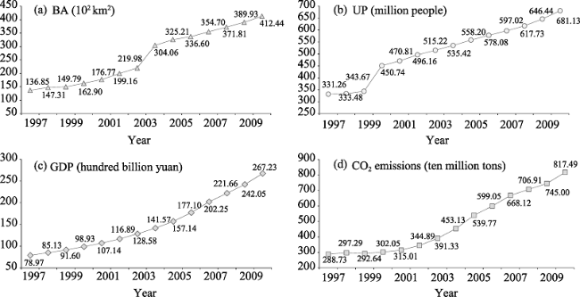
Figure 1 The changes in land urbanization (a), demographic urbanization (b), GDP (c) and CO2 emissions (d) for China between 1997 and 2010 |
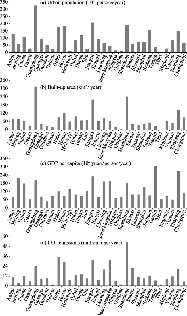
Figure 2 The growth rate in urban population (a), built-up area (b), GDP per capita (c) and CO2 emissions (d) for China’s 31 provinces |
Table 2 Panel unit root test results |
| Levels | |||||
|---|---|---|---|---|---|
| Variable | LLC | IPS | Fisher-ADF | Fisher-PP | |
| Intercept | BA | -2.75*** | 4.04 | 18.88 | 26.12 |
| UP | -4.68*** | 1.19 | 61.71 | 112.52*** | |
| pGDP | 5.863 | 12.1 | 9.23 | 4.24 | |
| CO2 | 1.65 | 7.18 | 8.4 | 6.45 | |
| Intercept and trend | BA | -1.50* | -1.47* | 47.28 | 52.87 |
| UP | -9.11*** | -0.27 | 67.02 | 27.63 | |
| pGDP | -10.31*** | -1.68** | 91.47*** | 68.99 | |
| CO2 | -6.39*** | -2.32** | 89.47** | 74.63 | |
| First differences | |||||
| Variable | LLC | IPS | Fisher-ADF | Fisher-PP | |
| Intercept | BA | -6.39*** | -4.65*** | 115.01*** | 224.74*** |
| UP | -11.32*** | -6.40*** | 149.70*** | 220.52*** | |
| pGDP | -4.51*** | -0.29 | 55.29** | 52.95*** | |
| CO2 | -6.12*** | -4.11*** | 106.59*** | 195.71*** | |
| Intercept and trend | BA | -5.54*** | -1.65*** | 75.35*** | 202.62*** |
| UP | -18.90*** | -9.45*** | 203.53*** | 309.78*** | |
| pGDP | -2.16*** | 0.42 | 59.99** | 105.29*** | |
| CO2 | -2.59*** | 0.10** | 53.40** | 158.00*** | |
Note: Newey-West bandwidth selection using Bartlett kernel. Automation selection of lags was based on SIC. Levin, Lin and Chu test (LLC) Null: unit root (assumes a common unit root process); Im, Pesaran and Shin W-stat test (IPSW), ADF-Fisher Chi-square test (ADF) and PP-Fisher Chi-square test (PP) Null: Unit root (assumes an individual unit root process). BA, UP, pGDP and CO2 are built-up area, urban population, and per capita GDP and CO2 emissions, respectively. The null hypothesis of the LLC, IPS, Fisher-ADF and Fisher PP tests examines non-stationary. ***, ** and * indicates statistical significance at the 1%, 5% and 10% significance level, respectively. |
Table 3 Panel cointegration test results |
| Statistics | Panel A | Panel B | Panel C | Panel D | Panel E |
|---|---|---|---|---|---|
| Panel v | 1.51* | 1.23 | 3.22*** | -0.03 | 3.70*** |
| Panel rho | -1.75** | 0.10 | -3.25*** | 0.71 | -1.93** |
| Panel PP | -2.40*** | -1.17 | -7.18*** | 0.24 | -5.31*** |
| Panel ADF | -2.98*** | -1.29* | -8.12*** | -1.19 | -8.10*** |
| Group rho | 1.48 | 2.77 | -0.35 | 2.67 | 0.13 |
| Group PP | -0.36* | 0.97 | -5.74*** | 0.96 | -5.63*** |
| Group ADF | -2.04** | -1.06* | -7.61*** | -1.26 | -8.80*** |
Note: Panel A (built-up area---pGDP); Panel B (urban population---pGDP); Panel C (built-up area---CO2); Panel D (urban population---CO2); Panel E (pGDP---CO2). Statistics are asymptotically distributed as normal. All tests contain only the intercept and not the trend term. The variance ratio test is right-side, which the others are left-sided. The null hypothesis is that the variables are not cointegrated. Lag length selected based on AIC automatically with a max lag of 2. ***, ** and * reject the null of no cointegration at the 1%, 5% and 10% significance level, respectively. |
Table 4 Panel cointegration coefficients by FMOLS and DOLS for China and its eastern, central and western regions |
| Whole China | |||||||
|---|---|---|---|---|---|---|---|
| Variable | Dependent variable: pGDP | Variable | Dependent variable: BA | ||||
| DOLS (1,1) | DOLS (2,2) | FMOLS | DOLS (1,1) | DOLS (2,2) | FMOLS | ||
| BA | 0.90*** (-27.29) | 0.81*** (-21.66) | 0.94*** (-27.58) | pGDP | 0.66*** (-9.64) | 0.22 (-0.47) | 0.93*** (-43.33) |
| Variable | Dependent variable: CO2 | Variable | Dependent variable: CO2 | ||||
| DOLS (1,1) | DOLS (2,2) | FMOLS | DOLS (1,1) | DOLS (2,2) | FMOLS | ||
| pGDP | 0.83*** (-16.22) | 0.60*** (-2.12) | 0.94*** (-61.07) | BA | 1.19*** (-36.78) | 1.16*** (-29.56) | 1.15*** (-34.88) |
| Obs | 341 | 279 | 403 | Obs | 341 | 279 | 403 |
| Eastern region | |||||||
| Variable | Dependent variable: pGDP | Variable | Dependent variable: BA | ||||
| DOLS (1,1) | DOLS (2,2) | FMOLS | DOLS (1,1) | DOLS (2,2) | FMOLS | ||
| BA | 1.02*** (-50.73) | 0.99*** (-6.63) | 1.03*** (-38.21) | pGDP | 0.66*** (-9.64) | 0.43 (-0.51) | 1.06*** (-26.07) |
| Variable | Dependent variable: CO2 | Variable | Dependent variable: CO2 | ||||
| DOLS (1,1) | DOLS (2,2) | FMOLS | DOLS (1,1) | DOLS (2,2) | FMOLS | ||
| pGDP | 0.90*** (-20.11) | 0.57 (-0.77) | 0.96*** (-42.37) | BA | 0.98*** (-75.43) | 0.99*** (-10.35) | 0.95*** (-45.29) |
| Obs | 121 | 99 | 143 | Obs | 121 | 99 | 143 |
| Central region | |||||||
| Variable | Dependent variable: pGDP | Variable | Dependent variable: BA | ||||
| DOLS (1,1) | DOLS (2,2) | FMOLS | DOLS (1,1) | DOLS (2,2) | FMOLS | ||
| BA | 1.17*** (-26.27 | 1.91*** (-52.62) | 1.21*** (-26.97) | pGDP | 0.90*** (-8.34) | 0.30 (-1.4) | 0.83*** (-25.16) |
| Variable | Dependent variable: CO2 | Variable | Dependent variable: CO2 | ||||
| DOLS (1,1) | DOLS (2,2) | FMOLS | DOLS (1,1) | DOLS (2,2) | FMOLS | ||
| pGDP | 0.64*** (-10.6) | 0.40*** (-4.28) | 0.84*** (-28.26) | BA | 0.99*** (-38.35) | 1.03*** (-28.1) | 0.98*** (-24.42) |
| Obs | 88 | 72 | 104 | Obs | 88 | 72 | 104 |
| Western region | |||||||
| Variable | Dependent variable: pGDP | Variable | Dependent variable: BA | ||||
| DOLS (1,1) | DOLS (2,2) | FMOLS | DOLS (1,1) | DOLS (2,2) | FMOLS | ||
| BA | 1.24*** (-32.66) | 1.35*** (-49.14) | 1.29*** (-28.75) | pGDP | 0.53*** (-5.90) | 0.25 (-1.92) | 0.79*** (-24.24) |
| Variable | Dependent variable: CO2 | Variable | Dependent variable: CO2 | ||||
| DOLS (1,1) | DOLS (2,2) | FMOLS | DOLS (1,1) | DOLS (2,2) | FMOLS | ||
| pGDP | 0.64*** (-7.24) | 0.63*** (-1.36) | 0.97*** (-29.77) | BA | 1.27*** (-43.92) | 1.29*** (-41.09) | 1.24*** (-27.96) |
| Obs | 88 | 72 | 104 | Obs | 88 | 72 | 104 |
Notes: BA and pGDP are built-up area and per capita GDP, respectively. The t-values are in parentheses. The panel method was grouped estimation. A panel data model with fixed effects was adopted. All tests were performed on the natural logarithm of the dependent and independent variables. Obs is observations. *, **and*** indicate the estimates are statistically significant at the 10%, 5% and 1% level, respectively. |
Table 5 Panel cointegration coefficients by FMOLS and DOLS for China based on the growth rate of all variables |
| Variable | Dependent variable: pGDP growth | Variable | Dependent variable: BA growth | ||||
|---|---|---|---|---|---|---|---|
| DOLS (1,1) | DOLS (2,2) | FMOLS | DOLS (1,1) | DOLS (2,2) | FMOLS | ||
| BA growth | 0.07 (1.29) | 0.04 (0.46) | 0.06 (3.16) | pGDP growth | -0.06 (-0.09) | 2.52 (1.13) | 0.62 (2.30) |
| Variable | Dependent variable: CO2 growth | Variable | Dependent variable: CO2 growth | ||||
| DOLS (1,1) | DOLS (2,2) | FMOLS | DOLS (1,1) | DOLS (2,2) | FMOLS | ||
| pGDP growth | 2.58*** (5.47) | 3.22** (2.00) | 1.76*** (7.01) | BA growth | 0.53*** (3.99) | 0.80*** (2.25) | 0.30*** (4.97) |
| Obs | 310 | 248 | 372 | Obs | 310 | 248 | 372 |
Notes: BA and pGDP are the growth rate of built-up area and per capita GDP, respectively. The t-values are in parentheses. The panel method was grouped estimation. A panel data model with fixed effects was adopted. All tests were performed on the natural logarithm of the dependent and independent variables. Obs is observations. **and*** indicate the estimates are statistically significant at the 5% and 1% level, respectively. |
Table 6 Wald F-test statistics based on panel-based vector error corrected models for the whole China and its eastern, central and western regions |
| Panel | Causal | Result | F-statistic value | |||
|---|---|---|---|---|---|---|
| Short-run causality | Long-run causality | |||||
| Whole China | A | pGDP | BA | 15.237 (0.00) | 192.31 (0.00) | |
| BA | pGDP | 7.204 (0.12) | 6421.924 (0.00) | |||
| B | BA | CO2 | 18.446 (0.00) | 313.338 (0.00) | ||
| CO2 | BA | 17.518 (0.10) | 194.408 (0.00) | |||
| C | pGDP | CO2 | 9.019 (0.05) | 6331.291 (0.00) | ||
| CO2 | pGDP | 4.444 (0.34) | 305.076 (0.00) | |||
| Eastern region | D | pGDP | BA | 0.635 (0.73) | 14.571 (0.01) | |
| BA | pGDP | 3.562 (0.17) | 28.332 (0.00) | |||
| E | BA | CO2 | 5.004 (0.05) | 8.156 (0.00) | ||
| CO2 | BA | 6.806 (0.16) | 19.042 (0.15) | |||
| F | pGDP | CO2 | 3.373 (0.04) | 10.885 (0.02) | ||
| CO2 | pGDP | 2.385 (0.30) | 59.190 (0.10) | |||
| Central region | G | pGDP | BA | 0.708 (0.70) | 12.490 (0.01) | |
| BA | pGDP | 3.116 (0.21) | 110.951 (0.00) | |||
| H | BA | CO2 | 10.981 (0.00) | 19.285 (0.00) | ||
| CO2 | BA | 3.562 (0.16) | 10.308 (0.12) | |||
| I | pGDP | CO2 | 2.640 (0.05) | 13.521 (0.00) | ||
| CO2 | pGDP | 12.367 (0.14) | 133.69 (0.10) | |||
| Western region | J | pGDP | BA | 0.231 (0.89) | 2.928 (0.71) | |
| BA | pGDP | 3.988 (0.13) | 53.577 (0.10) | |||
| K | BA | CO2 | 2.112 (0.35) | 6.898 (0.22) | ||
| CO2 | BA | 3.018 (0.22) | 6.749 (0.15) | |||
| L | pGDP | CO2 | 1.749 (0.42) | 4.501 (0.34) | ||
| CO2 | pGDP | 1.086 (0.58) | 169.38 (0.34) | |||
Notes: The null hypothesis is non-causality. BA, pGDP and CO2 are built-up area, per capita GDP and CO2 emissions, respectively. Cases with probability levels (shown in parentheses) lower than 0.05 reject the null hypothesis. |
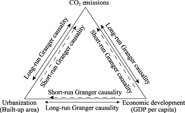
Figure 3 Long- and short-run Granger causality between land urbanization, economic growth and CO2 emissions in China |
Table 7 Heterogeneous panel Granger causality test results for the China and its eastern and western regions |
| Panel | Causal | Result | Wald-static | Zbar-static | Probability | |
|---|---|---|---|---|---|---|
| Whole China | A | pGDP | BA | Lag 1: 2.052 | Lag 1: 2.063 | 0.04 |
| Lag 2: 5.458 | Lag 2: 3.460 | 0.00 | ||||
| BA | pGDP | Lag 1: 3.743 | Lag 1: 6.411 | 0.10 | ||
| Lag 2: 3.207 | Lag 2: 0.530 | 0.60 | ||||
| B | BA | CO2 | Lag 1: 10.190 | Lag 1: 22.990 | 0.00 | |
| Lag 2: 10.792 | Lag 2: 10.403 | 0.00 | ||||
| CO2 | BA | Lag 1: 1.537 | Lag 1: 0.739 | 0.46 | ||
| Lag 2: 3.742 | Lag 2: 1.226 | 0.22 | ||||
| C | pGDP | CO2 | Lag 1: 7.138 | Lag 1: 15.143 | 0.00 | |
| Lag 2: 12.426 | Lag 2: 12.531 | 0.00 | ||||
| CO2 | pGDP | Lag 1: 1.789 | Lag 1: 1.386 | 0.17 | ||
| Lag 2: 4.363 | Lag 2: 2.035 | 0.04 | ||||
| Eastern region | Panel | Causal | Result | W-static | Zbar-stat | Porb. |
| D | pGDP | BA | Lag 1: 1.729 | Lag 1: 0.735 | 0.46 | |
| Lag 2:3.052 | Lag 2: 0.196 | 0.84 | ||||
| BA | pGDP | Lag 1: 3.643 | Lag 1: 3.665 | 0.00 | ||
| Lag 2: 7.598 | Lag 2: 3.721 | 0.00 | ||||
| E | BA | CO2 | Lag 1: 9.610 | Lag 1: 12.806 | 0.00 | |
| Lag 2: 7.604 | Lag 2: 3.725 | 0.00 | ||||
| CO2 | BA | Lag 1: 1.514 | Lag 1: 0.404 | 0.69 | ||
| Lag 2: 3.502 | Lag 2: 0.554 | 0.59 | ||||
| F | CO2 | pGDP | Lag 1: 0.953 | Lag 1: -0.454 | 0.65 | |
| Lag 2: 3.680 | Lag 2: 0.683 | 0.49 | ||||
| pGDP | CO2 | Lag 1: 6.039 | Lag 1: 7.336 | 0.00 | ||
| Lag 2: 15.939 | Lag 2: 10.189 | 0.00 | ||||
| Western region | Panel | Causal | Result | W-static | Zbar-stat | Porb. |
| J | pGDP | BA | Lag 1: 2.006 | Lag 1: 0.987 | 0.32 | |
| Lag 2: 5.319 | Lag 2: 1.666 | 0.10 | ||||
| BA | pGDP | Lag 1: 4.519 | Lag 1: 4.271 | 0.10 | ||
| Lag 2: 5.262 | Lag 2: 1.628 | 0.10 | ||||
| K | BA | CO2 | Lag 1: 7.959 | Lag 1: 8.765 | 0.09 | |
| Lag 2: 11.269 | Lag 2: 5.601 | 0.25 | ||||
| CO2 | BA | Lag 1: 1.566 | Lag 1: 0.412 | 0.68 | ||
| Lag 2: 1.266 | Lag 2: -0.014 | 0.31 | ||||
| L | CO2 | pGDP | Lag 1: 1.643 | Lag 1:0.513 | 0.61 | |
| Lag 2: 4.694 | Lag 2: 1.252 | 0.21 | ||||
| pGDP | CO2 | Lag 1: 8.808 | Lag 1: 9.873 | 0.35 | ||
| Lag 2: 13.559 | Lag 2: 7.114 | 0.68 |
Notes: The null hypothesis is homogeneous non-causality. Cases with probability levels lower than 0.05 reject the null hypothesis. Lag 1 and Lag 2 represent the test models of the Dumitrescu and Hurlin (2012) causality tests of lag order 1 and 2, respectively. |
Table 8 Hausman test results |
| Test summary | Chi-Sq. statistic | |
|---|---|---|
| Chi-Sq. statistic | Quadratic | Cubic |
| 40.304 | 41.210 | |
| Prob. | 0.000 | 0.000 |
| Accept model | Fixed effects | Fixed effects |
Table 9 Estimation results in pGDP and CO2 emissions based on the panel OLS estimator |
| Dependent variable [ln (CO2)] | Quadratic model | Cubic model | ||||
|---|---|---|---|---|---|---|
| Coefficient | t-statistic | Prob. | Coefficient | t-statistic | Prob. | |
| ln(pGDP) | 0.674 | 3.054 | 0.000 | -6.336 | -2.402 | 0.017 |
| ln(pGDP)2 | -0.003 | -0.184 | 0.854 | 0.997 | 2.657 | 0.008 |
| ln(pGDP)3 | - | -0.047 | -2.666 | 0.008 | ||
| ln(BA) | 0.293 | 8.239 | 0.000 | 0.286 | 8.089 | 0.000 |
| Constant | -1.717 | -2.247 | 0.025 | 14.589 | 2.368 | 0.018 |
| Turning point | - | (127.41, 10201.29) | ||||
| F-statistic | 597.542 | 0.000 | 589.035 | 0.000 | ||
| Adjusted R2 | 0.980 | 0.980 | ||||
| Wald test | H0: the quadratic model; H1:the cubic curve | |||||
| Wald statistic | 7.110*** | |||||
Note: Fixed effect OLS estimator was used. The number of samples was 434. “***” indicates the estimator of a parameter is significant at the 1% level. |
Table 10 Comparison with the other studies |
| Source | Data type | Method | Result |
|---|---|---|---|
| Jalil and Mahmud, 2009 | China; Time series (1975-2005) | ARDL, quadratic model; VECM; EKC hypothesis | Inverted U-shaped, GDP→CO2 |
| Wang et al., 2011 | China’s 28 provinces; panel data (1995-2007) | Pedroni cointegration; Panel VECM; EKC hypothesis | U-shaped curve; GDP→CO2 (long-run) |
| Du et al., 2012 | China’s 28 provinces; panel data (1995-2009) | Quadratic and cubic models; EKC hypothesis; GMM estimator | Inverted U-shaped is not strongly supported |
| Wang et al., 2012a | Beijing; Time series (1997-2010) | STIRPAT; OLS | Not support for EKC |
| This study | China’s 31 provinces; panel data (1997-2010) | Pedroni cointegration; Panel VECM; EKC hypothesis; OLS; cubic model | Long-run: BA↔GDP; BA↔CO2; GDP↔CO2; short-run: GDP→BA; BA→CO2; GDP→CO2; inverted N-shaped curve |
Note: ARDL refers to the auto regressive distributed lag; GMM represents the generalized method of moment; OLS is the ordinary least square; and STIRPAT refers to the stochastic impacts by regression on population, affluence and technology. The symbol “↔”, “→” represent the bidirectional and unidirectional Granger causality, respectively. |
The authors have declared that no competing interests exist.
| 1 |
|
| 2 |
|
| 3 |
|
| 4 |
|
| 5 |
|
| 6 |
|
| 7 |
|
| 8 |
|
| 9 |
|
| 10 |
|
| 11 |
|
| 12 |
|
| 13 |
|
| 14 |
|
| 15 |
|
| 16 |
|
| 17 |
|
| 18 |
|
| 19 |
|
| 20 |
International Energy Agency (IEA), 2012. Key world energy statistics international energy agency. Statistics Division, Paris.
|
| 21 |
|
| 22 |
|
| 23 |
|
| 24 |
|
| 25 |
|
| 26 |
|
| 27 |
|
| 28 |
|
| 29 |
|
| 30 |
|
| 31 |
|
| 32 |
|
| 33 |
|
| 34 |
|
| 35 |
|
| 36 |
|
| 37 |
National Bureau of Statistics of China (NBSC), 2011. China Statistical Yearbook 2011. Beijing: China Statistics Press.
|
| 38 |
|
| 39 |
|
| 40 |
|
| 41 |
|
| 42 |
|
| 43 |
|
| 44 |
|
| 45 |
|
| 46 |
|
| 47 |
|
| 48 |
|
| 49 |
|
| 50 |
|
| 51 |
Xinhua News Agency (XNA), 2011. The left-behind elderly reached more than 40 million. Xinhua News Agency Available from: [Accessed on 7 August 2014]
|
| 52 |
|
| 53 |
|
| 54 |
|
| 55 |
|
| 56 |
|
| 57 |
|
| 58 |
|
/
| 〈 |
|
〉 |