
Journal of Geographical Sciences >
Spatially distributed modelling and mapping of soil organic carbon and total nitrogen stocks in the Eastern Mau Forest Reserve, Kenya
Author: Kennedy Were, PhD, specialized in application of GIS and remote sensing techniques in environmental research. E-mail: kenwerez@yahoo.com
Received date: 2015-02-18
Accepted date: 2015-06-12
Online published: 2016-01-25
Copyright
Detailed knowledge about the estimates and spatial patterns of soil organic carbon (SOC) and total nitrogen (TN) stocks is fundamental for sustainable land management and climate change mitigation. This study aimed at: (1) mapping the spatial patterns, and (2) quantifying SOC and TN stocks to 30 cm depth in the Eastern Mau Forest Reserve using field, remote sensing, geographical information systems (GIS), and statistical modelling approaches. This is a critical ecosystem offering essential services, but its sustainability is threatened by deforestation and degradation. Results revealed that elevation, silt content, TN concentration, and Landsat 8 Operational Land Imager band 11 explained 72% of the variability in SOC stocks, while the same factors (except silt content) explained 71% of the variability in TN stocks. The results further showed that soil properties, particularly TN and SOC concentrations, were more important than that other environmental factors in controlling the observed patterns of SOC and TN stocks, respectively. Forests stored the highest amounts of SOC and TN (3.78 Tg C and 0.38 Tg N) followed by croplands (2.46 Tg C and 0.25 Tg N) and grasslands (0.57 Tg C and 0.06 Tg N). Overall, the Eastern Mau Forest Reserve stored approximately 6.81 Tg C and 0.69 Tg N. The highest estimates of SOC and TN stocks (hotspots) occurred on the western and northwestern parts where forests dominated, while the lowest estimates (coldspots) occurred on the eastern side where croplands had been established. Therefore, the hotspots need policies that promote conservation, while the coldspots need those that support accumulation of SOC and TN stocks.
Kennedy WERE , Bal Ram SINGH , Øystein Bjarne DICK . Spatially distributed modelling and mapping of soil organic carbon and total nitrogen stocks in the Eastern Mau Forest Reserve, Kenya[J]. Journal of Geographical Sciences, 2016 , 26(1) : 102 -124 . DOI: 10.1007/s11442-016-1257-4
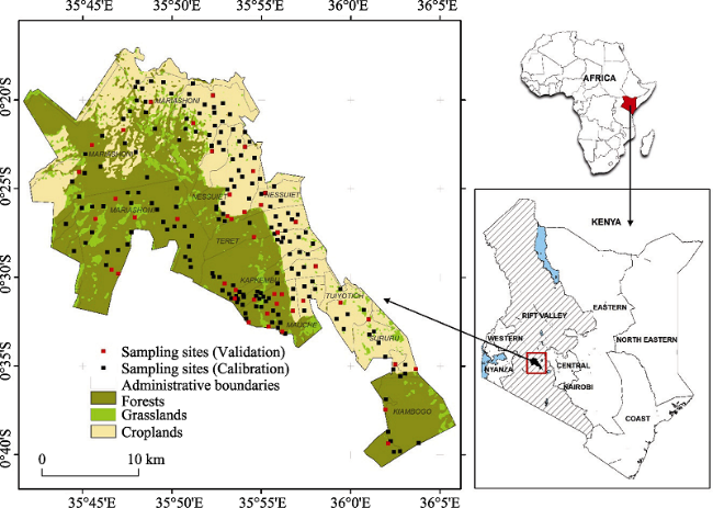
Figure 1 Geographical location of the study area |
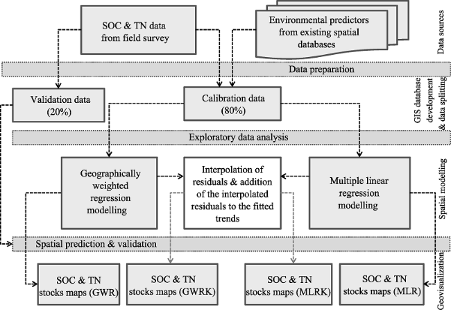
Figure 2 Illustration of the data sources and modelling framework |
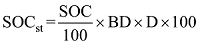
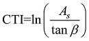
Table 1 Properties of the environmental predictors for spatial modelling |
| Variables | Data format | Date | Source | Scale | Soil-forming factor |
|---|---|---|---|---|---|
| Target variables | |||||
| 1. SOC stocks | Points | 2012 | Field work | ||
| 2. TN stocks | Points | 2012 | Field work | ||
| Predictor variables | |||||
| 1. SOC concentration | Raster | 2012 | Interpolated field data | 30 m | S |
| 2. TN concentration | Raster | 2012 | Interpolated field data | 30 m | S |
| 3. Magnesium | Raster | 2012 | Interpolated field data | 30 m | S |
| 4. Potassium | Raster | 2012 | Interpolated field data | 30 m | S |
| 5. Calcium | Raster | 2012 | Interpolated field data | 30 m | S |
| 6. Clay content | Raster | 2012 | Interpolated field data | 30 m | S |
| 7. Silt content | Raster | 2012 | Interpolated field data | 30 m | S |
| 8. Sand content | Raster | 2012 | Interpolated field data | 30 m | S |
| 9. pH | Raster | 2012 | Interpolated field data | 30 m | S |
| 10. Elevation | Raster | - | ASTER GDEM http://gdem.ersdac.jspacesystems.or.jp/ | 30 m | R |
| 11. Slope | Raster | - | ASTER GDEM | 30 m | R |
| 12. Aspect | Raster | - | ASTER GDEM | 30 m | R |
| 13. Curvature | Raster | - | ASTER GDEM | 30 m | R |
| 14. CTI | Raster | - | ASTER GDEM | 30 m | S |
| 15. Temperature | Raster | 1950-2000 | www.worldclim.org | 1 km | C |
| 16. Rainfall | Raster | 1950-2000 | www.worldclim.org | 1 km | C |
| 17. Surface reflectance & thermal emission | Raster | 30.05.2013 | Landsat 8 OLI (bands 2, 3, 4, 5, 6, 7, 10 & 11) http://earthexplorer.usgs.gov/ | 30 m | C, S |
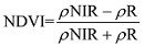
| 18. NDVI | Raster | 30.05.2013 | Landsat 8 OLI (bands 4 & 5) | 30 m | O |
| 19. PC bands | Raster | 30.05.2013 | Landsat 8 OLI (bands 2, 3, 4, 5, 6 & 7) | 30 m | S |
| 20. Land cover | Raster | 17.01.2011 | Landsat 5 TM; Were et al. (2013) | 30 m | O |
Note: SOC=soil organic carbon; TN=total nitrogen; CTI=compound topographic index; NDVI=normalized difference vegetation index; PC= principal component; S=soil properties; C=climate; O=organisms; and, R=topography |
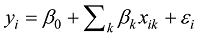

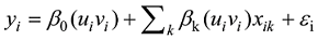
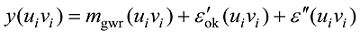
 is the estimated value, yi is the measured value, and n is the number of measured values in the testing data. The ME should be close to zero, while RMSE should be as small as possible. Average ME and RMSE values of the ten-fold validation are reported in this paper. Statistical validation was supplemented by visual inspection of the spatial patterns of the target variables.
Table 2 Descriptive statistics of SOC and TN stocks (0-30 cm) |
| Variable | n | Mean | Median | SD | CV (%) | Min. | Max. | Range | Skewness | Kurtosis |
|---|---|---|---|---|---|---|---|---|---|---|
| SOCst | 220 | 102.7 | 103.2 | 24.6 | 23.9 | 42.0 | 193.4 | 151.4 | 0.39 | 0.97 |
| TNst | 220 | 10.3 | 10.3 | 2.4 | 23.8 | 4.2 | 19.1 | 14.9 | 0.28 | 0.76 |
SD=standard deviation; CV=coefficient of variation; n=number of observations |
Table 3 Pearson’s correlation coefficient between the predictors and target variables selected for spatial modelling |
| Variables | 1 | 2 | 3 | 4 | 5 | 6 | 7 | 8 | 9 | 10 | 11 | 12 | 13 | 14 | 15 |
|---|---|---|---|---|---|---|---|---|---|---|---|---|---|---|---|
| 1. SOC stock | 1.00 | ||||||||||||||
| 2. TN stock | 0.99 | 1.00 | |||||||||||||
| 3. TN content | 0.84 | 0.85 | 1.00 | ||||||||||||
| 4. SOC content | 0.85 | 0.84 | 0.99 | 1.00 | |||||||||||
| 5. Silt | -0.41 | -0.42 | -0.56 | -0.55 | 1.00 | ||||||||||
| 6. Magnesium | 0.35 | 0.35 | 0.44 | 0.44 | -0.36 | 1.00 | |||||||||
| 7. Clay | 0.28 | 0.29 | 0.40 | 0.39 | -0.61 | 0.08 | 1.00 | ||||||||
| 8. Temperature | -0.50 | -0.50 | -0.63 | -0.63 | 0.28 | -0.04 | -0.34 | 1.00 | |||||||
| 9. Rainfall | 0.44 | 0.45 | 0.56 | 0.55 | -0.23 | 0.25 | 0.10 | -0.61 | 1.00 | ||||||
| 10. Elevation | 0.51 | 0.51 | 0.65 | 0.65 | -0.30 | 0.06 | 0.35 | -0.99 | 0.65 | 1.00 | |||||
| 11. Aspect | 0.22 | 0.23 | 0.18 | 0.17 | -0.08 | 0.01 | 0.02 | -0.16 | 0.16 | 0.16 | 1.00 | ||||
| 12. NDVI | 0.30 | 0.30 | 0.39 | 0.39 | -0.25 | 0.07 | 0.24 | -0.50 | 0.25 | 0.50 | 0.11 | 1.00 | |||
| 13. Land cover | -0.48 | -0.48 | -0.54 | -0.53 | 0.31 | 0.00 | -0.41 | 0.83 | -0.46 | -0.84 | -0.16 | -0.56 | 1.00 | ||
| 14. PC1 | -0.48 | -0.48 | -0.52 | -0.52 | 0.15 | -0.03 | -0.23 | 0.71 | -0.50 | -0.73 | -0.28 | -0.32 | 0.74 | 1.00 | |
| 15. Landsat 8 OLI band 11 | -0.58 | -0.58 | -0.65 | -0.65 | 0.35 | -0.09 | -0.37 | 0.81 | -0.56 | -0.84 | -0.29 | -0.63 | 0.89 | 0.82 | 1.00 |
Note: SOC=soil organic carbon; TN=total nitrogen; NDVI=normalized difference vegetation index; PC= principal component. Bold form shows that the correlation coefficient between the predictors and target variables exceeded the threshold value (r > 0.2). |
Table 4 Parameter estimates of the MLR models |
| Parameter | SOC stocks model | TN stocks model | ||||||||
|---|---|---|---|---|---|---|---|---|---|---|
| Estimate | SE | t value | Pr (>|t|) | VIF | Estimate | SE | t value | Pr (>|t|) | VIF | |
| Intercept | 143.502 | 50.757 | 2.827 | 0.0053** | - | 16.741 | 5.131 | 3.263 | 0.0013** | - |
| Silt | 0.443 | 0.202 | 2.191 | 0.0298* | 1.531 | - | - | - | - | - |
| Band 11 | -0.003 | 0.001 | -2.360 | 0.0194* | 3.511 | -0.000 | 0.000 | -2.475 | 0.0143* | 3.489 |
| Elevation | -0.022 | 0.009 | -2.503 | 0.0133* | 3.613 | -0.002 | 0.001 | -2.305 | 0.0223* | 3.558 |
| TN | 178.200 | 12.269 | 14.524 | 0.0000*** | 2.471 | - | - | - | - | - |
| SOC | - | - | - | - | - | 1.597 | 0.106 | 15.103 | 0.0000*** | 1.807 |
| Adjusted R2 | 0.72 | 0.71 | ||||||||
| RMSE | 13.07 | 1.33 | ||||||||
| Moran’s I | 0.11 | 0.08 | ||||||||
Significance codes: 0 '***' 0.001 '**' 0.01 '*' |
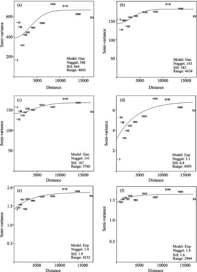
Figure 3 (a) Experimental variograms (points) and fitted models (lines) of SOC stocks (b) MLRsoc residuals (c) GWRsoc residuals (d) TN stocks (e) MLRtn residuals, and (f) GWRtn residuals |
Table 5 Parameter estimates of the GWR models |
| Parameter | SOC stocks model | TN stocks model | ||||||||
|---|---|---|---|---|---|---|---|---|---|---|
| Mean | SD | Min. | Max. | Range | Mean | SD | Min. | Max. | Range | |
| Intercept | 129.525 | 31.412 | 50.031 | 199.881 | 149.851 | 14.790 | 4.771 | 8.037 | 26.423 | 18.387 |
| Silt | 0.436 | 0.115 | 0.203 | 0.614 | 0.411 | - | - | - | - | - |
| Band 11 | -0.003 | 0.001 | -0.004 | -0.001 | 0.004 | -0.000 | 0.000 | -0.000 | -0.000 | 0.000 |
| Elevation | -0.021 | 0.007 | -0.041 | -0.004 | 0.037 | -0.002 | 0.001 | -0.005 | -0.001 | 0.004 |
| TN | 177.230 | 23.072 | 142.790 | 238.558 | 95.768 | - | - | - | - | - |
| SOC | - | - | - | - | - | 1.576 | 0.197 | 1.087 | 1.899 | 0.812 |
| Global adjusted R2 | 0.73 | 0.72 | ||||||||
| Global RMSE | 12.86 | 1.29 | ||||||||
| Moran’s I | 0.06 | 0.02 | ||||||||
Table 6 Parameters of the fitted variogram models for SOC and TN stocks, and the residuals of the respective GWR and MLR models |
| Variable | Model | Nugget Mg ha-1 | Partial sill Mg ha-1 | Total sill Mg ha-1 | Range (m) | Nugget- to- sill ratio (%) | Spatial dependence |
|---|---|---|---|---|---|---|---|
| SOC stocks | Gaussian | 386 | 278 | 664 | 4845 | 58.1 | Moderate |
| MLRsoc residuals | Gaussian | 143 | 39 | 182 | 4434 | 78.6 | Weak |
| GWRsoc residuals | Gaussian | 141 | 26 | 167 | 5760 | 84.4 | Weak |
| TN stocks | Exponential | 3.1 | 3.7 | 6.8 | 4493 | 45.6 | Moderate |
| MLRtn residuals | Exponential | 1.4 | 0.5 | 1.9 | 4132 | 73.7 | Weak |
| GWRtn residuals | Exponential | 1.4 | 0.2 | 1.6 | 2944 | 87.5 | Weak |
Table 7 Summary statistics of the spatial prediction errors |
| SOCst (Mg C ha-1) | TNst (Mg N ha-1) | |||
|---|---|---|---|---|
| ME | RMSE | ME | RMSE | |
| GWRK | -0.48 | 16.74 | 0.04 | 1.53 |
| GWR | -0.86 | 16.66 | -0.03 | 1.51 |
| MLRK | 0.39 | 19.42 | -0.31 | 1.93 |
| MLR | 0.30 | 19.89 | -0.33 | 1.93 |
ME= mean error; RMSE=root mean squared error |
Table 8 Soil organic carbon and nitrogen stocks under different land cover types |
| Land cover | Area | SOC stocks | TN stocks | |||||||
|---|---|---|---|---|---|---|---|---|---|---|
| Min. | Max. | Mean | Total | Min. | Max. | Mean | Total | |||
| (Ha) | (Mg ha-1) | (Tg) | (Mg ha-1) | (Tg) | ||||||
| Forests | 32228.4 | 75.5 | 142.9 | 110.4 | 3.78 | 7.5 | 15.3 | 11.1 | 0.38 | |
| Grasslands | 5509.4 | 66.7 | 129.8 | 103.5 | 0.57 | 6.7 | 12.6 | 10.4 | 0.06 | |
| Croplands | 25828.1 | 62.9 | 126.9 | 95.2 | 2.46 | 6.5 | 12.2 | 9.6 | 0.25 | |
| Total | 65565.9 | 6.81 | 0.69 | |||||||
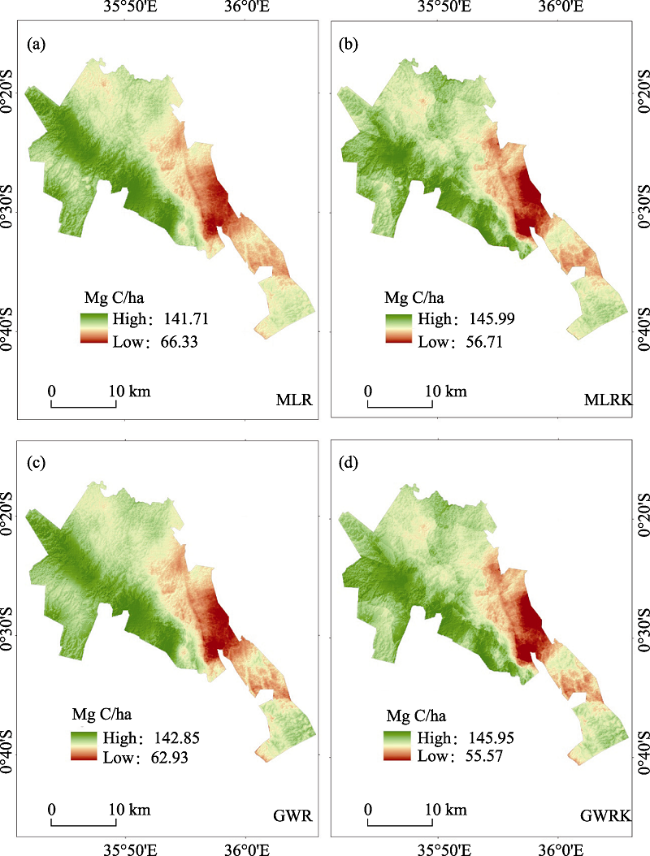
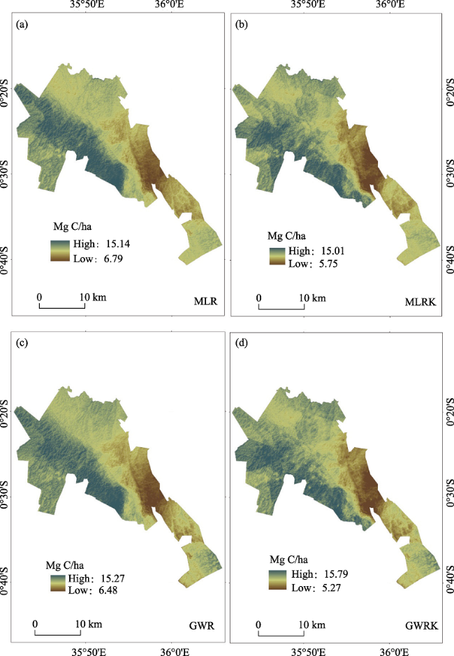
Figure 4 Maps showing the spatial patterns of the predicted SOC stocks using MLR, MLRK, GWR and GWRK |
Figure 5 Maps showing the spatial patterns of the predicted TN stocks using MLR, MLRK, GWR and GWRK |
The authors have declared that no competing interests exist.
| 1 |
|
| 2 |
|
| 3 |
|
| 4 |
|
| 5 |
|
| 6 |
|
| 7 |
|
| 8 |
|
| 9 |
|
| 10 |
|
| 11 |
|
| 12 |
|
| 13 |
|
| 14 |
|
| 15 |
|
| 16 |
|
| 17 |
[Accessed 2014, January 19].
|
| 18 |
|
| 19 |
|
| 20 |
|
| 21 |
|
| 22 |
IPCC, 2006. IPCC Guidelines for national greenhouse gas inventories, prepared by the national greenhouse gas inventories programme, Eggleston H S, Buendia L, Miwa K et al. (eds.). Published: IGES, Japan.
|
| 23 |
|
| 24 |
|
| 25 |
|
| 26 |
|
| 27 |
|
| 28 |
|
| 29 |
|
| 30 |
|
| 31 |
|
| 32 |
|
| 33 |
|
| 34 |
|
| 35 |
|
| 36 |
|
| 37 |
|
| 38 |
|
| 39 |
|
| 40 |
|
| 41 |
|
| 42 |
|
| 43 |
|
| 44 |
|
| 45 |
|
| 46 |
|
| 47 |
|
| 48 |
|
| 49 |
|
| 50 |
|
| 51 |
|
| 52 |
|
| 53 |
|
| 54 |
|
| 55 |
|
| 56 |
|
| 57 |
|
| 58 |
|
| 59 |
|
| 60 |
|
| 61 |
|
| 62 |
|
| 63 |
|
| 64 |
|
| 65 |
|
| 66 |
|
| 67 |
|
| 68 |
|
| 69 |
|
| 70 |
UNEP, 2009[Accessed 2013, August 28].
|
| 71 |
|
| 72 |
|
| 73 |
|
| 74 |
|
| 75 |
|
| 76 |
|
| 77 |
|
| 78 |
|
| 79 |
|
| 80 |
|
| 81 |
|
| 82 |
|
| 83 |
|
| 84 |
|
| 85 |
|
| 86 |
|
/
| 〈 |
|
〉 |