
Journal of Geographical Sciences >
Scenario simulation and landscape pattern dynamic changes of land use in the PovertyBelt around Beijing and Tianjin: A case study of Zhangjiakou city, Hebei Province
Author: Sun Piling (1984-), PhD Candidate, specialized in land use/cover change, sustainable utilization of land resources. E-mail:sapphire816@163.com
*Corresponding author: Xu Yueqing (1972-), PhD and Associate Professor, E-mail:xmoonq@sina.com
Received date: 2015-04-15
Accepted date: 2015-10-12
Online published: 2016-03-20
Supported by
National Natural Science Foundation of China, No.41171088, No.41571087
Copyright
Land use/cover change has been recognized as a key component in global change and has attracted increasing attention in recent decades. Scenario simulation of land use change is an important issue in the study of land use/cover change, and plays a key role in land use prediction and policy decision. Based on the remote sensing data of Landsat TM images in 1989, 2000 and 2010, scenario simulation and landscape pattern analysis of land use change driven by socio-economic development and ecological protection policies were reported in Zhangjiakou city, a representative area of the Poverty Belt around Beijing and Tianjin. Using a CLUE-S model, along with socio-economic and geographic data, the land use simulation of four scenarios-namely, land use planning scenario, natural development scenario, ecological-oriented scenario and farmland protection scenario-were explored according to the actual conditions of Zhangjiakou city, and the landscape pattern characteristics under different land use scenarios were analyzed. The results revealed the following: (1) Farmland, grassland, water body and unused land decreased significantly during 1989-2010, with a decrease of 11.09%, 2.82%, 18.20% and 31.27%, respectively, while garden land, forestland and construction land increased over the same period, with an increase of 5.71%, 20.91% and 38.54%, respectively. The change rate and intensity of land use improved in general from 1989 to 2010. The integrated dynamic degree of land use increased from 2.21% during 1989-2000 to 3.96% during 2000-2010. (2) Land use changed significantly throughout 1989-2010. The total area that underwent land use change was 4759.14 km2, accounting for 12.53% of the study area. Land use transformation was characterized by grassland to forestland, and by farmland to forestland and grassland. (3) Under the land use planning scenario, farmland, grassland, water body and unused land shrank significantly, while garden land, forestland and construction land increased. Under the natural development scenario, construction land and forestland increased in 2020 compared with 2010, while farmland and unused land decreased. Under the ecological-oriented scenario, forestland increased dramatically, which mainly derived from farmland, grassland and unused land. Under the farmland protection scenario, farmland was well protected and stable, while construction land expansion was restricted. (4) The landscape patterns of the four scenarios in 2020, compared with those in 2010, were more reasonable. Under the land use planning scenario, the landscape pattern tended to be more optimized. The landscape became less fragmented and heterogeneous with the natural development scenarios. However, under the ecological-oriented scenario and farmland protection scenario, landscape was characterized by fragmentation, and spatial heterogeneity of landscape was significant. Spatial differences in landscape patterns in Zhangjiakou city also existed. (5) The spatial distribution of land use could be explained, to a large extent, by the driving factors, and the simulation results tallied with the local situations, which provided useful information for decision-makers and planners to take appropriate land management measures in the area. The application of the combined Markov model, CLUE-S model and landscape metrics in Zhangjiakou city suggests that this methodology has the capacity to reflect the complex changes in land use at a scale of 300 m×300 m and can serve as a useful tool for analyzing complex land use driving factors.
Key words: land use change; Markov model; CLUE-S model; landscape metrics; Zhangjiakou city
SUN Piling , XU Yueping , YU Zhonglei , LIU Qingguo , XIE Baopeng , LIU Jia . Scenario simulation and landscape pattern dynamic changes of land use in the PovertyBelt around Beijing and Tianjin: A case study of Zhangjiakou city, Hebei Province[J]. Journal of Geographical Sciences, 2016 , 26(3) : 272 -296 . DOI: 10.1007/s11442-016-1268-1
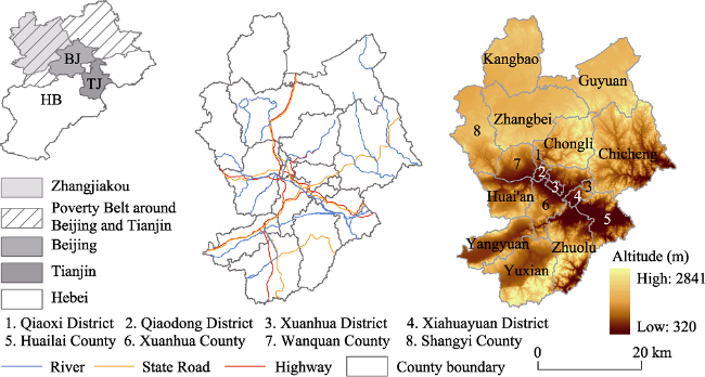
Figure 1 Location of the study area and its elevation |
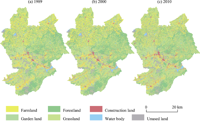
Figure 2 Land use pattern in Zhangjiakou city throughout 1989-2010 |
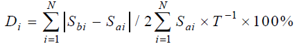
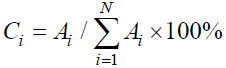
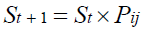

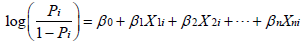
Table 1 Values of land use type conversion elasticity (ELAS) in Zhangjiakou city |
| Relative elasticity | Farmland | Garden land | Forestland | Grassland | Construction land | Water body | Unused land |
|---|---|---|---|---|---|---|---|
| Land use planning scenario | 0.7 | 0.9 | 0.8 | 0.8 | 0.9 | 0.9 | 0.5 |
| Natural development scenario | 0.8 | 0.8 | 0.8 | 0.9 | 0.9 | 0.9 | 0.4 |
| Ecological-oriented scenario | 0.8 | 0.9 | 0.9 | 0.9 | 0.9 | 0.9 | 0.6 |
| Farmland protection scenario | 0.9 | 0.9 | 0.9 | 0.9 | 0.9 | 0.9 | 0.8 |
Table 2 Land use changes in Zhangjiakou city throughout 1989-2010 |
| Land use types | 1989 | 2010 | 1989-2010 | |||
|---|---|---|---|---|---|---|
| Area (km2) | Proportion (%) | Area (km2) | Proportion (%) | Change area (km2) | Change rate (%) | |
| Farmland | 10900.30 | 29.61 | 9691.74 | 26.33 | -1208.56 | -11.09 |
| Garden land | 1412.81 | 3.84 | 1493.49 | 4.06 | 80.68 | 5.71 |
| Forest land | 9149.40 | 24.86 | 11062.80 | 30.06 | 1913.4 | 20.91 |
| Grassland | 11207.94 | 30.45 | 10891.42 | 29.59 | -316.52 | -2.82 |
| Construction land | 1000.24 | 2.72 | 1385.73 | 3.77 | 385.49 | 38.54 |
| Water body | 963.16 | 2.62 | 787.84 | 2.14 | -175.32 | -18.20 |
| Unused land | 2171.62 | 5.90 | 1492.45 | 4.05 | -679.17 | -31.27 |
Table 3 Rate of land use change during different periods in Zhangjiakou city |
| Periods | Land use dynamic degree (%) | Integrated dynamic degree (%) | ||||||
|---|---|---|---|---|---|---|---|---|
| Farmland | Garden land | Forest land | Grassland | Construction land | Water body | Unused land | ||
| 1989-2000 | -0.27 | 0.51 | 0.56 | -0.15 | 1.32 | -0.88 | -0.73 | 2.21 |
| 2000-2010 | -0.83 | 0.01 | 1.39 | -0.11 | 2.10 | -0.94 | -2.53 | 3.96 |
Table 4 Main types of land use change in Zhangjiakou city throughout 1989-2010 |
| 1989-2000 | 2000-2010 | 1989-2010 | |||
|---|---|---|---|---|---|
| Transformation type | Ci (%) | Transformation type | Ci (%) | Transformation type | Ci (%) |
| Grassland to Forestland | 29.61 | Grassland to Forestland | 27.69 | Grassland to Forestland | 29.15 |
| Farmland to Grassland | 18.67 | Farmland to Forestland | 17.83 | Farmland to Forestland | 16.26 |
| Farmland to Forestland | 8.05 | Grassland to Farmland | 10.96 | Grassland to Farmland | 11.30 |
| Unused land to Forestland | 6.65 | Unused land to Grassland | 10.09 | Unused land to Forestland | 8.44 |
| Farmland to Construction land | 6.21 | Unused land to Forestland | 8.55 | Unused land to Grassland | 8.21 |
| Grassland to Farmland | 5.17 | Farmland to Construction land | 5.67 | Farmland to Construction land | 6.04 |
| Unused land to Grassland | 4.16 | Farmland to Garden land | 3.65 | Farmland to Garden land | 4.21 |
| Other 31 types | 21.48 | Other 43 types | 15.56 | Other 36 types | 16.39 |
| Total | 100.00 | Total | 100.00 | Total | 100.00 |
Table 5 Logistic regression results of the spatial distribution of land use types in Zhangjiakou city throughout 2000-2010 |
| Drivers | Farmland | Garden land | Forestland | Grassland | Construction land | Water body | Unused land | |||||||
|---|---|---|---|---|---|---|---|---|---|---|---|---|---|---|
| β | EXP(β) | β | EXP(β) | β | EXP(β) | β | EXP(β) | β | EXP(β) | β | EXP(β) | β | EXP(β) | |
| X1 | -0.0228 | 0.9775 | 0.0117 | 1.0118 | 0.0250 | 1.0253 | 0.0117 | 1.0118 | -0.0453 | 0.9557 | -0.0730 | 0.9296 | — | — |
| X2 | — | — | — | — | -0.0340 | 0.9666 | 0.0441 | 1.0451 | — | — | — | — | — | — |
| X3 | -0.0009 | 0.9991 | -0.0093 | 0.9908 | 0.0008 | 0.9992 | 0.0227 | 1.0229 | -0.0026 | 0.9974 | -0.0020 | 0.9980 | 0.0185 | 1.0187 |
| X4 | -0.2729 | 0.7612 | -0.4639 | 0.6288 | 0.0345 | 1.0351 | -0.1669 | 0.8463 | -0.197 | 0.8212 | 0.0276 | 1.0280 | 0.0415 | 1.0424 |
| X5 | 0.0006 | 1.0006 | — | — | — | — | -0.0005 | 0.9995 | — | — | — | — | — | — |
| X6 | -0.0065 | 0.9935 | 0.0568 | 1.0585 | -0.0120 | 0.9881 | 0.0154 | 1.0155 | -0.0163 | 0.9839 | -0.0545 | 0.9470 | — | — |
| X7 | -0.0083 | 0.9917 | 0.0435 | 1.0445 | 0.0100 | 1.0100 | -0.0066 | 0.9935 | -0.0189 | 0.9813 | — | — | -0.0024 | 0.9976 |
| X8 | -0.0285 | 0.9719 | — | — | 0.0269 | 1.0272 | — | — | -0.1232 | 0.8841 | 0.0999 | 1.1051 | -0.1026 | 0.9025 |
| X9 | — | — | -0.0472 | 0.9539 | 0.0055 | 1.0055 | 0.0019 | 1.0019 | — | — | 0.0106 | 1.0106 | -0.0159 | 0.9843 |
| X10 | — | — | — | — | — | — | 0.009 | 1.0091 | — | 0.9998 | — | — | -0.0852 | 0.9183 |
| X11 | -0.0009 | 0.9991 | 0.0015 | 1.0015 | -0.0008 | 0.9992 | -0.0007 | 0.9993 | -0.0002 | — | — | — | — | — |
| X12 | -0.0282 | 0.9722 | 0.0354 | 1.0360 | -0.0297 | 0.9707 | -0.0046 | 0.9954 | — | — | — | — | -0.1562 | 0.8554 |
| X13 | 0.0007 | 1.0007 | -0.0018 | 0.9982 | -0.0002 | 0.9998 | -0.0004 | 0.9996 | 0.0004 | 1.0004 | — | — | 0.0014 | 1.0014 |
| X14 | 0.0044 | 1.0045 | 0.0074 | 1.0074 | -0.0034 | 0.9966 | -0.0038 | 0.9962 | 0.0014 | 1.0014 | — | — | 0.0243 | 1.0246 |
| X15 | -0.0001 | 0.9999 | 0.0004 | 1.0004 | — | — | — | — | — | — | 0.0002 | 1.0002 | -0.0002 | 0.9998 |
| Constant | -0.1458 | 0.8643 | -12.7820 | 0.0001 | -8.7846 | 0.0002 | -9.8221 | 0.0001 | -4.4890 | 0.0112 | -2.0367 | 0.1305 | -9.9562 | 0.0014 |
| ROC value | 0.896 | 0.878 | 0.870 | 0.862 | 0.915 | 0.835 | 0.798 | |||||||
Note: The mark “—” denotes the factors removed. X1-landform, X2-soil organic matter, X3-elevation, X4-slope, X5-aspect, X6-distance to the nearest river, X7-distance to the nearest town center, X8-distance to the nearest county center, X9-distance to the nearest main road, X10-distance to the nearest railway, X11-population density, X12-urbanization rate, X13-economic density, X14-fixed assets investment, X15-per-capita net income of farmers. |
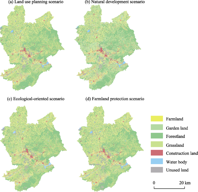
Table 6 The prediction results of land use under different scenarios (km2) |
| Year | Scenario design | Farmland | Garden land | Forestland | Grassland | Construction land | Water body | Unused land |
|---|---|---|---|---|---|---|---|---|
| 2010 | Actual land use | 9691.74 | 1493.49 | 11062.80 | 10891.42 | 1385.73 | 787.84 | 1492.45 |
| 2020 | Land use planning scenario | 8721.00 | 1500.49 | 12932.90 | 10634.90 | 1535.00 | 725.48 | 755.70 |
| Natural development scenario | 8288.79 | 1521.89 | 13061.68 | 10819.07 | 1744.20 | 722.96 | 646.88 | |
| Ecological-oriented scenario | 8844.12 | 1495.98 | 12478.14 | 10756.97 | 1521.87 | 728.66 | 979.73 | |
| Farmland protection scenario | 9429.17 | 1562.82 | 11543.47 | 10712.17 | 1516.48 | 712.91 | 1328.45 |
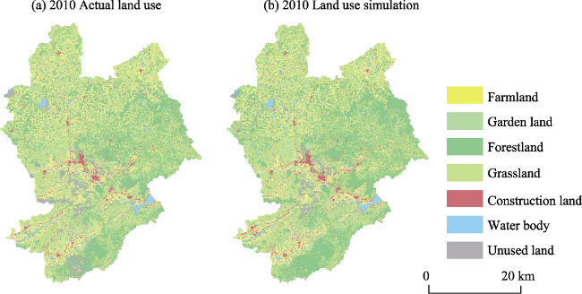
Figure 3 Land use map (a) and simulation map (b) of Zhangjiakou city in 2010 |
Figure 4 Land use simulation maps of Zhangjiakou city in 2020 |
Table 7 Landscape metrics of Zhangjiakou city under different scenarios |
| Land use scenario | F | LSI | PAFRAC | SHDI | IJI | CONTAG | AI |
|---|---|---|---|---|---|---|---|
| 2010 Actual land use | 0.0097 | 131.4746 | 1.5738 | 1.5691 | 73.8408 | 29.6276 | 59.4424 |
| Land use planning scenario (Reference scenario) | 0.0090 | 126.4539 | 1.5730 | 1.5875 | 73.9858 | 32.2885 | 61.0127 |
| Natural development scenario | 0.0089 | 126.6271 | 1.5768 | 1.5519 | 73.2345 | 32.5534 | 60.9583 |
| Ecological-oriented scenario | 0.0093 | 128.0227 | 1.5744 | 1.5706 | 72.5546 | 31.1907 | 60.5223 |
| Farmland protection scenario | 0.0095 | 129.8600 | 1.5750 | 1.5733 | 70.5517 | 30.0865 | 59.9485 |
Table 8 Class metrics of Zhangjiakou city under different scenarios |
| Farmland | Garden land | Forestland | Grassland | Construction land | Water body | Unused land | ||
|---|---|---|---|---|---|---|---|---|
| 2010 Actual land use | F | 0.0055 | 0.0177 | 0.0068 | 0.0076 | 0.0447 | 0.0377 | 0.0181 |
| PAFRAC | 1.6025 | 1.5709 | 1.5594 | 1.6022 | 1.4809 | 1.5045 | 1.4974 | |
| LSI | 127.6094 | 67.2558 | 126.8260 | 141.3391 | 82.5360 | 51.7500 | 57.0814 | |
| Land use planning Scenario (Reference scenario) | F | 0.0048 | 0.0176 | 0.0057 | 0.0079 | 0.0427 | 0.0345 | 0.0204 |
| PAFRAC | 1.5989 | 1.5712 | 1.5613 | 1.6038 | 1.4983 | 1.5014 | 1.5112 | |
| LSI | 118.6083 | 66.3977 | 123.0988 | 141.0610 | 85.2759 | 47.5944 | 44.5054 | |
| Natural development scenario | F | 0.0048 | 0.0170 | 0.0054 | 0.0076 | 0.0417 | 0.0340 | 0.0182 |
| PAFRAC | 1.6003 | 1.5693 | 1.5667 | 1.6028 | 1.5134 | 1.4991 | 1.5189 | |
| LSI | 116.2158 | 63.9960 | 125.3124 | 141.2334 | 90.3011 | 46.9441 | 40.1000 | |
| Ecological-oriented scenario | F | 0.0049 | 0.0177 | 0.0059 | 0.0077 | 0.0434 | 0.0339 | 0.0214 |
| PAFRAC | 1.5992 | 1.5727 | 1.5622 | 1.6033 | 1.5106 | 1.4971 | 1.5078 | |
| LSI | 119.4530 | 66.4690 | 123.6671 | 141.1055 | 89.5018 | 46.3911 | 50.6555 | |
| Farmland protection scenario | F | 0.0052 | 0.0170 | 0.0066 | 0.0077 | 0.0435 | 0.0342 | 0.0195 |
| PAFRAC | 1.6008 | 1.5731 | 1.5595 | 1.6031 | 1.4988 | 1.4941 | 1.5091 | |
| LSI | 124.5201 | 67.0455 | 124.7448 | 140.7728 | 85.5211 | 46.1638 | 56.3827 | |
The authors have declared that no competing interests exist.
| [1] |
|
| [2] |
|
| [3] |
|
| [4] |
|
| [5] |
|
| [6] |
|
| [7] |
|
| [8] |
|
| [9] |
|
| [10] |
|
| [11] |
|
| [12] |
|
| [13] |
|
| [14] |
|
| [15] |
|
| [16] |
|
| [17] |
|
| [18] |
|
| [19] |
|
| [20] |
|
| [21] |
|
| [22] |
|
| [23] |
|
| [24] |
|
| [25] |
|
| [26] |
|
| [27] |
|
| [28] |
|
| [29] |
|
| [30] |
|
| [31] |
|
| [32] |
|
| [33] |
|
| [34] |
|
| [35] |
|
| [36] |
|
| [37] |
|
| [38] |
|
| [39] |
|
| [40] |
|
| [41] |
|
| [42] |
|
| [43] |
|
| [44] |
|
| [45] |
|
| [46] |
|
| [47] |
|
| [48] |
|
| [49] |
|
| [50] |
|
| [51] |
|
| [52] |
|
| [53] |
|
| [54] |
|
| [55] |
|
| [56] |
|
| [57] |
|
| [58] |
|
| [59] |
|
| [60] |
|
| [61] |
|
| [62] |
|
| [63] |
|
| [64] |
|
| [65] |
|
| [66] |
|
| [67] |
|
| [68] |
|
| [69] |
|
| [70] |
|
| [71] |
|
| [72] |
|
| [73] |
|
| [74] |
|
| [75] |
|
/
| 〈 |
|
〉 |