Orginal Article

Simulating urban land use change by incorporating an autologistic regression model into a CLUE-S model

  • JIANG Weiguo , 1, 2 ,
  • CHEN Zheng 1, 2 ,
  • LEI Xuan , 3, * ,
  • JIA Kai 1, 2 ,
  • WU Yongfeng 4
Expand
  • 1. State Key Laboratory of Earth Surface Processes and Resource Ecology, Beijing Normal University, Beijing 100875, China
  • 2. Key Laboratory of Environmental Change and Natural Disaster, Beijing Normal University, Beijing 100875, China
  • 3. Tianjin University Research Institute of Urban Planning, Tianjin 300073, China
  • 4. Institute of Environment and Sustainable Development in Agriculture, Chinese Academy of Agricultural Sciences, Beijing 100081, China

*Corresponding author: Lei Xuan (1988-), MS, E-mail:

Author: Jiang Weiguo (1976-), Associate Professor, specialized in ecological remote sensing and natural hazard and risk analysis. E-mail:

Received date: 2014-12-17

  Accepted date: 2015-02-12

  Online published: 2015-06-24

Supported by

National Natural Science Foundation of China, No.41171318

National Key Technology Support Program, No.2012BAH32B03;No.2012BAH33B05

Special Fund for Forest Scientific Research in the Public Welfare, No.201204201

Copyright

Journal of Geographical Sciences, All Rights Reserved

Abstract

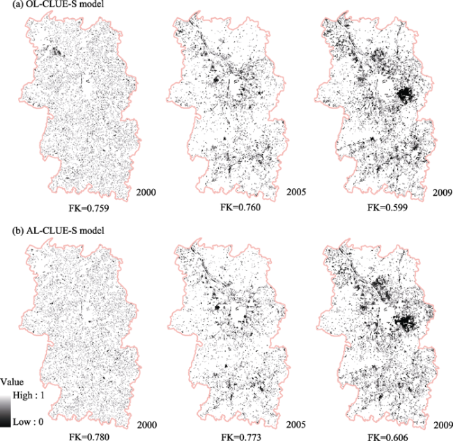
The Conversion of Land Use and its Effects at Small regional extent (CLUE-S) model is a widely used method to simulate land use change. An ordinary logistic regression model was integrated into the CLUE-S model to identify explanatory variables without considering the spatial autocorrelation effect. Using image-derived maps of the Changsha- Zhuzhou-Xiangtan urban agglomeration, the CLUE-S model was integrated with the ordinary logistic regression and autologistic regression models in this paper to simulate land use change in 2000, 2005 and 2009 based on an observation map from 1995. Significant positive spatial autocorrelation was detected in residuals of ordinary logistic models. Some variables that were much more significant than they should be were selected. Autologistic regression models, which used autocovariate incorporation, were better able to identify driving factors. The Receiver Operating Characteristic Curve (ROC) values of autologistic regression models were larger than 0.8 and the pseudo R2 values were improved, compared with results of logistic regression model. By overlapping the observation maps, the Kappa values of the ordinary logistic regression model (OL)-CLUE-S and autologistic regression model (AL)-CLUE-S models were larger than 0.75. The results showed that the simulation results were indeed accurate. The Kappa fuzzy (Kfuzzy) values of the AL-CLUE-S models (0.780, 0.773, 0.606) were larger than the values of the OL-CLUE-S models (0.759, 0.760, 0.599) during the three periods. The AL-CLUE-S models performed better than the OL-CLUE-S models in the simulation of land use change. The results showed that it is reasonable to integrate autocovariates into CLUE-S models. However, the Kfuzzy values decreased with prolonged duration of simulation and the maximum range of time was not discussed in this paper.

Cite this article

JIANG Weiguo , CHEN Zheng , LEI Xuan , JIA Kai , WU Yongfeng . Simulating urban land use change by incorporating an autologistic regression model into a CLUE-S model[J]. Journal of Geographical Sciences, 2015 , 25(7) : 836 -850 . DOI: 10.1007/s11442-015-1205-8

1 Introduction

The land use types have been changing due to the rapid urbanization in China. There are a variety of factors which impact the pattern of Chinese urban development (Liu et al., 2014). Scholars often use spatial change models to simulate and predict land use change in order to understand the reasons and progress of land use conversion (Liu et al., 2014; Koomen et al., 2008; He et al., 2005; Verburg et al., 2004).
At present, the Cellular Automata (CA) model (He et al., 2005; Kuang et al., 2011; Wu et al., 2009), the Conversion of Land Use and its Effects (CLUE) model as well as the Conversion of Land Use and its Effects at Small regional extent (CLUE-S) model are the most commonly used models to study land use change. The CLUE model, a dynamic model to simulate the conversion of land use and its effects, was presented by Veldkamp et al. (1996). It has been widely and successfully used for the simulation of land use changes over continents, countries, etc. (DE Koning et al., 1999; Verburg et al., 2000). The work of Veldkamp et al. showed that the CLUE model was superior to the biophysical equilibrium models for the prediction of future land cover (Veldkamp and Fresco, 1996). On the basis of the CLUE model, Verburg et al. developed the CLUE-S model to analyse land use change at a small scale (Verburg et al., 2002). Verburg et al. used a global economic model and an integrated assessment model to calculate changes in demand for the European Union, and simulated the future spatial pattern of the European mainland in different economic development situations (Verburg et al., 2008). The CLUE-S model has been widely used in the simulated study of land use conversion at a regional scale (Bai et al., 2005; Cai et al., 2004; Guo et al., 2012; Zhu et al., 2010; Zheng et al., 2014).
Land use change simulation is a complicated process, which is determined by the interaction of spatial and temporal factors such as natural, social and economic, etc. (Zhou and He, 2007). A thorough analysis and revelation of the interrelationships between land spatial distribution and driving factors is the premise and foundation of land use spatial simulation (Veldkamp and Fresco, 1997). Ordinary logistic regression models, which are integrated into the CLUE-S model, are commonly used to select the driving factors of land use change, including biophysical and socio-economic variables (Verburg et al., 2002; Gong et al., 2014; Xie and Li, 2008). It assumes that the data is statistically independent and identically distributed. However, the spatial land use data has the tendency to be dependent (Overmars et al., 2003). The assumption does not take into account the spatial autocorrelation existing in the spatial data. The standard error of the statistical tests could therefore be underestimated, resulting in an increasing in Type 1 errors. With spatial autocorrelation being ignored, the importance of variables, which have little or no relevance to the response variables, might be overestimated (Overmars et al., 2003). Consequently, the selected driving forces and simulation results could be inaccurate (Wu et al., 2009; Wu et al., 2010). The autologistic model proposed by Besag incorporating the spatial autocorrelation factor into the ordinary logistic model (Besag, 1972), can solve the problem of the spatial autocorrelation effect existing in spatial statistical analysis. It had been widely used in the ecological diversity modelling (Wu et al., 2009; Wu and Huffer, 1997). However, there is a lack of in-depth study in terms of land use spatial simulation (Triantakonstantis et al., 2013).
Based on related researches, this paper chose Changsha-Zhuzhou-Xiangtan (Chang-Zhu- Tan) urban agglomeration in China as the study area. The ordinary logistic regression model (OL) and autologistic regression model (AL) were integrated respectively with the CLUE-S model to simulate the regional land use spatial distribution pattern in 2000, 2005 and 2009 based on the land use data. Environment variables and the socio-economic factors were used to identify explanatory factors. The observed maps(years of 2000, 2005,2009)from remote sensing images were used to validate the precision of the models. The importance of considering the spatial autocorrelation factor in the simulated change of urban land use will be discussed by comparing the performance of the ordinary logistic-CLUE-S (OL-CLUE-S) model and the autologistic-CLUE-S (AL-CLUE-S) model.

2 Study area and data

2.1 Study area

The study area is Chang-Zhu-Tan urban agglomeration, which consists of planned urban areas of Changsha, Zhuzhou and Xiangtan in Hunan Province. It is located in the middle and lower reaches of the Xiangjiang River (Figure 1), between 112°38’-113°17’E and 37°38’-28°33’N, with an area of 4588 km2. Terrain in the study area is mainly composed of low mountains, hills, lowland and flood plains. It is rich in mineral resources. The main soil type of the region is red soil, and the natural production potential is excellent. The Chang-Zhu-Tan region is an important economic tie, which connects the northern and southern cities together. The Chang-Zhu-Tan urban agglomeration has the highest level of industrialization and urbanization, and the highest density of population, compared with other cities in Hunan province. The spatial structure is compact and the centrality of Changsha, Zhuzhou and Xiangtan is getting significantly. The Chang-Zhu-Tan urban agglomeration has been expanding constantly and the urbanization rate had increased by 11.8% from 2001 to 2006 (Zeng et al., 2012). Its population was as high as 13.57 million in 2010.
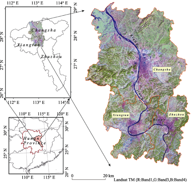
Figure 1 Location of the study area

2.2 Data

2.2.1 Remote sensing data
The remote sensing data used in this paper were Landsat data acquired in November 1995 (TM), December 2000 (ETM+), October 2005 (TM) and December 2009 (TM). Based on previous urban land use classification systems and spectral characteristics of the Landsat TM/ETM image, built-up area, wetland, green land, bare land and cultivated land were identified and selected as training samples. The remote sensing data were classified using the SVM (Support Vector Machine) method and resampled to 300 m × 300 m. The accuracy assessment results showed that the Kappa indexes for each time period for cultivated land, built-up area and wetland, etc. were larger than 0.8, and the Kappa index for green land was 0.75. The overall accuracy of classification conformed to the requirement of the study. The observed land use map for 1995 was shown as Figure 2a and the observed maps of 2000, 2005 and 2009 were shown as Figure 4.
The observed land use map of 1995 was used as the basal input data. The observed maps of 2000, 2005 and 2009 were the basic data for the calculation of land use change demanded area and for accuracy assessment.
2.2.2 Collection of explanatory variables
Driving factors not only included commonly used factors for land use change, but also included other factors in light of the certain regional characteristics. According to the characteristics of terrain, water, geographical and transportation advantages, environment variables such as slope, aspect and elevation were selected as the typical biophysical factors, and the minimum distances to roads, rivers and residential area were selected as the typical socio-economic factors. Therefore, Chang-Zhu-Tan traffic data (1:50000; Figure 2b), terrain data (1:50000; Figure 2c), regional river system map (Figure 2d), settlements data (Figure 2e), soil type map and the Chang-Zhu-Tan land use statistical data were selected as source data to identify explanatory factors. The spatial distributions of 15 factors were calculated using the shortest Euclidean distance method. The 15 factors were distance from stations (DS), distance from city centres (DC), distance from urban centre (DU), distance from main country settlements (DCS), distance from county centre (DCT), distance from expressway (DEW), distance from railway (DRW), distance from village road (DVR), distance from county border (DCR), distance from the Xiangjiang River (DX), distance from branches of the Xiangjiang River (DBX), elevation, slope, aspect and soil types.
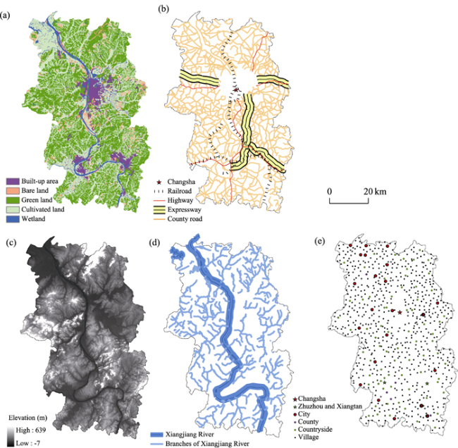
Figure 2 The observation map for 1995 (a); Spatial distribution of traffic system (b); DEM of Chang-Zhu-Tan megalopolis (c); Distribution of river network (d); Distribution of settlements (e)

3 Methods

3.1 The CLUE-S model

The CLUE-S model is used to establish the statistical relationship between land use spatial distribution and driving factors in order to analyse land use scenarios based on systems theory. First, an assumption is established: the demand for area of different land use types, in a given area, is an important driving force, and the relationship between the total demand area, regional natural environment, socio-economic situation and land use spatial pattern remains in a dynamic equilibrium.
The CLUE-S model includes two distinct modules, namely a non-spatial demand module and a spatially explicit allocation procedure. The non-spatial analysis module calculates changes in area of all land use types in a certain period of time based on analysis of natural, social and economic factors, or in areas of each type over a given time period. The spatial analysis module translates these demands into land use changes at appropriate locations according to the impacted spatial characteristics of land use types, and produces the land use spatial simulation (Wang et al., 2010). The study unit of the CLUE-S model is a grid. To reflect spatial information at a high resolution on the premise of appropriate accuracy, the grid size for this paper was 300 m × 300 m.
The CLUE-S model requires inputting the transfer matrix of possible conversion between various land use types. All of the five land use types in this article can change into other types, with the exception of urban land which cannot change into itself, bare land, green land or wetland.

3.2 Logistic and autologistic regression models

In this study, ordinary logistic regression and autologistic regression models were used to identify driving factors. To establish a land use spatial distribution prediction model based on ordinary logistic regression models, the study area was initially subdivided into a number of space (grid) units. The response variable (the spatial distribution of land use type) was expressed by a binary presence (where 1 indicated that transition occurred, and 0 indicated that the class did not exist and explanatory variables would be described by some biophysical and socio-economic factors). The ordinary logistic regression model is defined as:
where pi is the probability of specified land use type (i) transition in the grid, and βi is a coefficient to be estimated for each explanatory variable Xn,i.
The autologistic model incorporated spatial dependence into the ordinary logistic regression model to eliminate the spatial autocorrelation effect. The conditional probability of a certain type in the grid unit (X, T) is defined as a function of various external variables and a variable of spatial relationship between grid units. The specific formula is as follows:
where autocov is the spatial autocorrelation variable. The autocov of grid i is determined by the formula:
where yj is the probability of a certain type existing in pixel j, 1 = exists, 0 = does not exist, wij is the weight coefficient according to the distance d between pixel i and pixel j, wij = 1/d when the distance between pixel i and pixel j, otherwise wij = 0.

3.3 Validation

3.3.1 Validation of regression results
The ROC (Relative Operating Characteristics) was designed to evaluate the ability of logistic regression models and it was widely used to verify the spatial change simulation models (Pontius and Schneider, 2001). The values of ROC are between 0.5-1. The greater the ROC values are, the more satisfactory the regression model is, and the higher accuracy of the spatial distribution of land use type is. It is generally believed when the ROC value varies between 0.5 and 0.7, the accuracy of the model is low; when the ROC value varies between 0.7 and 0.9, the accuracy is credible; and when the ROC value is larger than 0.9, the model has a high precision (Manel et al., 2001).
Nagelkerke’s R2 (which is an index attempting to imitate R2 in the linear regression model based on the likelihood value) reflects the closeness of fit of regression models (Nagelkerke, 1991). Generally, the greater the index is, the greater proportion is explained by the model, and the higher accuracy of the model prediction is.
The Moran's I coefficient suggests the similarity of spatial proximity pixel values (Moran, 1950). Moran's I is used to describe the spatial autocorrelation characteristics of ordinary logistic regression and autologistic regression residuals. Moran’s I usually varies between -1 and 1. When the value is between -1 and 0, the space is negative correlation; when the value is between 0 and 1, the space is positive correlation; when Moran’s I is 0, there is no correlation and the residuals distribute randomly in space.
3.3.2 Validation of land use simulation results
The Kappa index and Fuzzy Kappa index (Kfuzzy) were used to assess the simulation results. The Kappa index evaluates model accuracy by comparing the actual data and the simulation results pixel by pixel (Pontius, 2000). According to Pontius (2002) and Hagen (2003), some similar landscape patterns and identical spatial pixels of two images could exist in a certain neighbouring extent. Therefore, Kfuzzy, whose formula format is the same as the Kappa index, is introduced to evaluate the accuracy of the simulation. Kfuzzy is a modified Kappa index, taking position ambiguity and type ambiguity in a neighbouring pixel extent.
where Po is the observed percentage of agreement, Pc is the expected random correct simulation ratio, Pc=1/n, n is the number of land use types, Pp is the correct ideal simulation ratio, Pp = 1, and Pe is the expected similarity, based upon given histograms.

4 Results

4.1 Logistic regression and autologistic regression results

The regression coefficients (B) and standard errors (S.E.) of variables are shown in Tables 1 and 2. Where ‘-’ represents ‘significance of variables are larger than 0.05’. If B is negative, the correlativity of land use change and driving factors is negative.
According to Tables 1 and 2, the number and types of variables of autologistic regression results were different from ordinary logistic regression results. Distance to stations, distance to city centres and distance to branches of the Xiangjiang River were not in the autologistic regression results, and aspect was selected as a variable. Because of the incorporation of the autocovariate, the autologistic model eliminated and modified some variables that were much more significant than they should be, and took into account some spatial factors that impacted land use change. The regression results showed that elevation was a common factor. The terrain factor was an important variable to land use spatial distribution and change in Chang-Zhu-Tan. In the study area, expressways were the main driving factor for land use change, soil type and village settlement location were important factors for green land and cultivated land change.
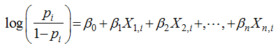
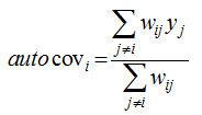
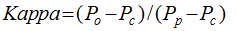
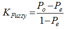
Table 1 Logistic regression results
Variables Built-up area Bare land Green land Wetland Cultivated land
B S.E. B S.E. B S.E. B S.E. B S.E.
DS (km) 0.086 0.021 0.04 0.01 -0.013 0.005 0.057 0.011 - -
DC (km) - - - - - - - - 0.011 0.004
DU (km) -0.039 0.011 - - - - 0.087 0.017 - -
DCS (km) 0.537 0.046 - - -0.184 0.049 - - -0.298 0.046
Elevation (m) -0.446 0.041 -0.062 0.029 1.303 0.042 -0.466 0.077 -1.075 0.042
DEW (km) -0.114 0.007 0.053 0.005 0.018 0.005 - - - -
Slope - - - - - - - - - -
Aspect - - 0.117 0.029 -0.134 0.039 - - - -
DRW (km) 0.058 0.013 - - 0.04 0.017 0.079 0.021 - -
DCT (km) -0.097 0.02 - - - - - - - -
DCR (km) 0.087 0.005 -0.01 0.004 - - 0.041 0.009 -0.042 0.005
DX (km) - - - - - - 0.122 0.035 - -
DBX (km) -0.127 0.011 - - - - -0.102 0.016 0.082 0.008
DVR (km) 0.117 0.034 -0.127 0.039 -0.079 0.036 0.107 0.055 - -
Soil type 0.212 0.057 - - -0.189 0.073 0.4 0.092 -0.255 0.066
Constant -0.108 0.02 - - - - - - -0.143 0.018
Table 2 Autologistic regression results
Variables Built-up area Bare land Green land Wetland Cultivated land
B S.E. B S.E. B S.E. B S.E. B S.E.
DS (km) - - - - - - - - - -
DC (km) - - - - - - - - - -
DU (km) - - - - - - 0.07 0.018 - -
DCS (km) - - - - -0.167 0.054 - - -0.214 0.049
Elevation (m) -0.357 0.05 -0.062 0.053 0.702 0.047 -0.218 0.071 -0.715 0.044
DEW (km) -0.038 0.007 0.053 0.008 - - - - - -
Slope 0.111 0.038 0.133 0.043 -0.077 0.03 - - 0.13 0.036
Aspect 0.072 0.021 - - - - 0.109 0.023 -0.052 0.017
DRW (km) - - -0.054 0.012 - - - - - -
DCT (km) - - - - - - - - -0.032 0.005
DCR (km) - - - - - - 0.123 0.035 - -
DX(km) - - 0.052 0.013 - - - - 0.066 0.008
DBX(km) - - - - - - - - - -
DVR (km) - - - - - - - - -0.17 0.074
Soil type -0.082 0.024 - - - - -0.156 0.04 -0.066 0.019
Autocovariate 8.819 0.285 18.94 0.706 3.993 0.164 8.133 0.581 3.16 0.16
Constant 0.399 0.489 -1.995 0.182 -3.088 0.147 1.067 0.79 1.995 0.459
The ROC and pseudo R2 values of logistic and autologistic regression results are shown in Table 3. The ROC values of autologistic regression results were larger than 0.8 and the pseudo R2 values were improved, compared to the logistic regression results. The regression models of urban were the best and the regression accuracy of bare land was substantially improved. According to ROC and pseudo R2 values, the autologistic regression model performed better than the ordinary logistic model. The autologistic regression model was better able to identify driving factors.
Table 3 The ROC and pseudo R2 of the logistic regression and autologistic regression results
Models Built-up area Bare land Green land Wetland Cultivated land
ROC R2 ROC R2 ROC R2 ROC R2 ROC R2
Logistic 0.847 0.455 0.628 0.264 0.823 0.385 0.770 0.269 0.769 0.395
Autologistic 0.941 0.701 0.833 0.481 0.865 0.504 0.847 0459 0.813 0.481
Moran’s I value for Pearson residuals of ordinary logistic and autologistic regression models at 600 m lag distance are shown in Figure 3. The Moran’s I values of the two models decreased with lag distance. Significant positive spatial autocorrelation existed in residuals of ordinary logistic models within a certain distance. The variables in the autologistic models were more explanatory and had a better goodness of fit than the ordinary logistic model. The spatial autocorrelation was insignificant in autologistic regression residuals so that the autologistic model had a better statistical stability and yielded more credible results.
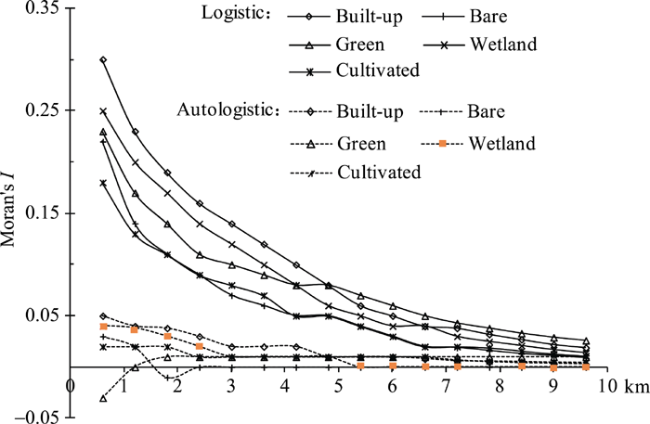
Figure 3 Moran’s I value for Pearson residuals of the logistic and autologistic regression models

4.2 Land use simulation results

The Chang-Zhu-Tan land use maps from 2000, 2005 and 2009 were simulated (based on an observed map from 1995) by both OL-CLUE-S model and AL-CLUE-S model. Variables and regression coefficients (B) were the input parameters. In this study, the Xiangjiang River and its branches were assumed to be unchanged. The simulation maps of built-up area, bare land, green land, wetland and cultivated land in 2000, 2005 and 2009 are shown in Figure 4.
According to the observed maps, the built-up area of Chang-Zhu-Tan was increasing and the spatial pattern was compacting. The simulation maps of the OL-CLUE-S and the AL-CLUE-S models showed similar results. The observed maps and simulation maps were the same as the real development in Chang-Zhu-Tan.
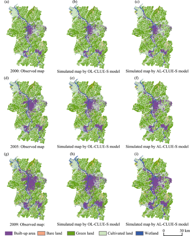
Figure 4 Simulated maps of the OL-CLUE-S and the AL-CLUE-S models and the observed maps of Chang-Zhu-Tan megalopolis of 2000, 2005 and 2009

4.3 Validation of land use simulation results

In this paper, the Kappa and Kfuzzy indexes were used to calculate spatial overlap in order to validate the accuracy of the simulation results. The values of Kfuzzy ranged from 0 to 1. If the value was 1, it suggested that the simulation map matched observed map perfectly. If the value was 0, it suggested that the simulation map was completely different from the observed map. By overlapping the observed maps, the Kappa values (Table 4) of the OL-CLUE-S and the AL-CLUE-S models were larger than 0.75. The results showed that the simulation results indicated considerable accuracy. The Kappa and Kfuzzy values (Figure 5) of the AL-CLUE-S model were larger than the values of the OL-CLUE-S model in three time periods. It suggested that the AL-CLUE-S model performed better for the simulation of land use change. However, the Kfuzzy values decreased with prolonged duration of simulation. The Kfuzzy values of the years 2000 and 2005 simulation maps were similar and larger than 0.75. While the Kfuzzy values for the 2005 and 2009 simulation maps were less than Kappa values. The differences were 0.16 and 0.17, respectively.
Table 4 The Kappa indexes of simulation results from 2000, 2005 and 2009
Model 2000 2005 2009
OL-CLUE-S 0.794 0.846 0.754
AL-CLUE-S 0.805 0.872 0.757
Figure 5 The simulated Fuzzy Kappa (FK) values of the OL-CLUE-S and the AL-CLUE-S models from 2000, 2005 and 2009

5 Discussion

The autologistic regression results had different and less variables comparing with ordinary logistic regression results. The ROC and pseudo R2 values suggested that the autologistic models were better able to explain dependent variables, and the results of autologistic models were more precise than the results of logistic models. Ordinary logistic models assumed that variables were independent and uniformly distributed. However, the residuals of ordinary logistic models were significant, which suggested that the assumption of independence was violated (Overmars et al., 2003). Because of the Type 1 error, some variables were overemphasised and their significance was overestimated. The Type 1 error could cause some bias of land use simulation results (Lennon, 2000). Zhou et al. (2011) combined CLUE-S models and Markov model to predict the land use change in Jiangsu Province and the accuracy was verified. However, the autocorrelation factor was not considered and the ROC values were very different among different land use types. The ROC values of dry land and paddy field were less than 0.8. The application of the autologistic regression model to land use change simulation was suggested to be more reasonable (Dai and Zhang, 2013; Wu et al., 2010). According to the regression results of OL and AL models, the distance from expressway and elevation were important to the development of Chang-Zhu-Tan urban agglomeration. Therefore, it was necessary to improve traffic environment. Besides, the roads should be away from wetland in order to protect wetland from being destroyed. Some socio-economic factors such as population density and GDP data were not included in the regression process due to the difficulty of collection. Therefore, the involvement of more factors and the consideration of dynamic driving factors in the discussion of the relationship between natural, societal and economic factors and their interactive relationships was a suggested direction for future research.
The Kfuzzy values of the AL-CLUE-S results, into which the spatial autocorrelation factor was incorporated, were larger than the OL-CLUE-S results. After the incorporation of autocovariate terms, the spatial interactions between the variables of land use change were adequately considered. The AL-CLUE-S model could reflect a truer process of change and effectively improve the simulation accuracy of the CLUE-S (Hubbell et al., 2001). The results of Wu et al. (2009) suggested that the ALCA models showed considerable improvement over the OLCA models. It was necessary to consider autocovariate terms in spatial change simulations. Urban agglomeration was a new spatial structure of urban development. Unordered urban expansion could be avoided and urban development structure could be more reasonably assessed by the incorporation of spatial autocovariates in urban planning. Autocovariates had a significant effect on the simulation of urban land use change.
Liu et al. (2009) employed CLUE-S model to simulate land use change in the upper reaches of the Minjiang River and the maximum simulation time range was 22 years. Batisani and Yarnal (2009) argued that the simulation accuracy of CLUE-S model was just 16% when the time range was 10 years. In this paper, the accuracy of the simulated landscape pattern maps of the OL-CLUE-S and the AL-CLUE-S models were considerable within ten years and when the range of time increased to 14 years, the accuracy started to decrease due to the uncertainty of the input parameters (Wu et al.,2012). The faster decreasing velocity of the AL-CLUE-S models suggested that the limits of the AL-CLUE-S were more significant than those of the OL-CLUE-S models. The AL-CLUE-S models were adapted to simulate land use change over a short period of time and, in practice, it was important to select the best simulated time range. Because of the limitation of remote sensing data, the decreasing velocity of simulation accuracy with time ranges was not included in this paper. The maximum time range for simulation was not defined. In future work, more remote sensing data of different time periods will be considered to assess and analyse simulation accuracy.

6 Conclusions

The study employed the AL-CLUE-S models and OL-CLUE-S models to simulate land use change of the Chang-Zhu-Tan urban agglomeration in 2000, 2005 and 2009. In this paper, spatial autocorrelation was considered and the regression and simulation results were compared with the results of the OL-CLUE-S models. The results showed that: (1) the selected variables were more reasonable and it was necessary to incorporate autocovariates into the land use change simulation model. According to ROC and pseudo R2 values, the autologistic regression model was more suitable for identifying driving factors. (2) The simulation maps of the AL-CLUE-S were more precise than the OL-CLUE-S based on regression results. The Kappa values of the AL-CLUE-S model were larger than 0.75 in three time periods. The Kfuzzy values of the AL-CLUE-S model were 0.780, 0.773 and 0.606 respectively in 2000, 2005 and 2009. Both of the Kappa and Kfuzzy values of the AL-CLUE-S models were larger than the values of the OL-CLUE-S models. It suggests that the AL-CLUE-S models were more appropriate for the simulation of land use change than the OL-CLUE-S model. (3)The accuracy of the simulation results in 2000 was the highest among the three time periods and the accuracy of simulation maps decreased with time range, especially from 2005 to 2009. This decrease suggested that the predictability of the CLUE-S could be influenced by the incorporation of autocovariates due to the uncertainty of the input parameters.

The authors have declared that no competing interests exist.

1
Bai Wanqi, Zhang Yongmin, Yan Jianzhonget al., 2005. Simulation of land use dynamics in the upper reaches of the Dadu river.Geographical Research, 24(2): 206-212. (in Chinese)

2
Batisani N, Yarnal B, 2009. Uncertainty awareness in urban sprawl simulations: Lessons from a small US metropolitan region. Land Use Policy, 26(2): 178-185.

3
Besag J, 1972. Nearest-neighbor systems and the auto-logistic model for binary data.Journal of the Royal Statistical Society B, 34(1): 75-83.

4
Cai Yumei, Liu Yansui, Yu Zhenronget al., 2004. Progress in spatial simulation of land use change: CLUE-S model and its application.Progress in Geography, 23(4): 63-71. (in Chinese)

5
Dai Shengpei, Zhang Bo, 2013. Land use change scenarios simulation in the middle reaches of the Heihe river basin based on CLUE-S model: A case of Ganzhou district of Zhangye city.Journal of Natural Resources, 28(2): 336-348. (in Chinese)

6
De Koning G H J, Verburg P H, Veldkamp Aet al., 1999. Multi-scale modelling of land use change dynamics in Ecuador.Agricultural Systems, 61(2): 77-93.

7
Gong Jianzhou, Chen Wenli, Liu Yansuiet al., 2014. The intensity change of urban development land: Implications for the city master plan of Guangzhou, China. Land Use Policy, 40: 91-100.

8
Guo Yanfeng, Yu Xiubo, Jiang Luguanget al., 2012. Scenarios analysis of land use change based on CLUE-S model in Jiangxi Province by 2030.Geographical Research, 31(6): 1016-1028. (in Chinese)

9
Hagen A E, 2003. Fuzzy set approach to assessing similarity of categorical maps.International Journal of Geographic Information Systems, 17(3): 235-249.

10
He Chunyang, Shi Peijun, Chen Jinet al., 2005. Developing land use scenario dynamics model by the integration of system dynamics model and cellular automata model.Science in China Ser. D Earth Sciences, 48(11): 1979-1989.

11
Hubbell S P, Ahumada J A, Condit Ret al., 2001. Local neighborhood effects on long-term survival of individual trees in a Neotropical forest. Ecological Research, 16(5): 859-875.

12
Koomen E, Rietveld P, De Nijs T, 2008. Modelling land-use change for spatial planning support.The Annals of Regional Science, 42(1): 1-10.

13
Kuang Wenhui, 2011. Simulation dynamic urban expansion at regional scale in Beijing-Tianjin-Tangshan metropolitan area.Journal of Geographical Sciences, 21(1): 317-330.

14
Lennon J J, 2000. Red-shifts and red herrings in geographical ecology. Ecography, 23(1): 101-113.

15
Liu Jiyuan, Kuang Wenhui, Zhang Zengxiang, et al., 2014. Spatiotemporal characteristics, patterns, and causes of land-use changes in China since the late 1980s.Journal of Geographical Sciences, 24(2): 195-210.

16
Liu Miao, Hu Manyuan, Chang Yuet al., 2009. Analysis of temporal predicting abilities for the CLUE-S land use model. Acta Ecologica Sinica, 29(11): 6110-6119. (in Chinese)

17
Liu Yan, Feng Yongjiu, Pontius R G, 2014. Spatially-explicit simulation of urban growth through self-adaptive genetic algorithm and cellular automata modelling. Land, 3(3): 719-738.

18
Manel S, Williams H C, Ormerod S J, 2001. Evaluating presence-absence models in ecology: The need to account for prevalence.Journal of Applied Ecology, 38(5): 921-931.

19
Moran P A P, 1950. Notes on continuous stochastic phenomena.Biometrika, 37(1/2): 17-23.

20
Nagelkerke N J D, 1991. A note on general definition of the coefficient of determination.Biometrika, 78(3): 691-692.

21
Overmars K P, De Koning G H J, Veldkamp A, 2003. Spatial autocorrelation in multi-scale land use models.Ecological Modelling, 164(2/3): 257-270.

22
Pontius R G, 2000. Quantification error versus location error in comparison of categorical map.Photogrammetric Engineering and Remote Sensing, 66(8): 1011-1016.

23
Pontius R G, 2002. Statistical methods to partition effects of quantity and location during comparison of categorical maps at multiple resolutions.Photogrammetric Engineering and Remote Sensing, 68(10): 1041-1049.

24
Pontius R G, Schneider L C, 2001. Land-cover change model validation by a ROC method for the Ipswich watershed, Massachusetts, USA. Agriculture, Ecosystems & Environment, 85(1-3): 239-248.

25
Triantakonstantis D P, Kalivas D P, Kollias V J, 2013. Autologistic regression and multicriteria evaluation models for the prediction of forest expansion. New Forests, 44(2): 163-181.

26
Veldkamp A, Fresco L O, 1996. CLUE: A conceptual model to study the conversion of land use and its effects. Ecological Modelling, 85(2/3): 253-270.

27
Veldkamp A, Fresco L O, 1997. Exploring land use scenarios: An alternative approach based on actual land use.Agricultural Systems, 55(1): 1-17.

28
Verburg P H, Chen Y Q, Veldkamp A, 2000. Spatial explorations of land use change and grain production in China.Agriculture, Ecosystems & Environment, 82(1-3): 333-354.

29
Verburg P H, Eickhout B, Van Meijl H, 2008. A multi-scale, multi-model approach for analyzing the future dynamics of European land use.The Annals of Regional Science, 42(1): 57-77.

30
Verburg P H, Schot P P, Dijst M Jet al., 2004. Land use change modelling: Current practice and research priorities.GeoJournal, 61(4): 309-324.

31
Verburg P H, Soepboer W, Veldkamp Aet al., 2002. Modeling the spatial dynamics of regional land use: The CLUE-S Model.Environmental Management, 30(3): 391-405.

32
Wang Liyan, Zhang Xueru, Zhang Huaet al., 2010. Principle and structure of CLUE-S model and its progress.Geography and Geo-information Science, 26(3): 73-77. (in Chinese)

33
Wu Daqian, Liu Jian, Zhang Gaoshenget al., 2009. Incorporating spatial autocorrelation into cellular automata model: An application to the dynamics of Chinese tamarisk.Ecological Modelling, 220(24): 3490-3498.

34
Wu Guiping, Zeng Yongnian, Xiao Pengfenget al., 2010. Using autologistic spatial models to simulate the distribution of land-use patterns in Zhangjiajie, Hunan Province.Journal of Geographical Sciences, 20(2), 310-320.

35
Wu Hulin, Huffer F W, 1997. Modelling the distribution of plant species using the autologistic regression model.Environmental and Ecological Statistics, 4(1): 49-64.

36
Wu Jiansheng, Feng Zhe, Gao Yanget al., 2012. Recent progresses on the application and improvement of CLUE-S model.Progress in Geography, 31(1): 3-10. (in Chinese)

37
Xie Hualin, Li Bo, 2008. Driving forces analysis of land-use pattern changes based on Logistic regression model in the farming-pastoral zone: A case study of Ongiud Banner, Inner Mongolia.Geographical Research, 27(2): 294-304. (in Chinese)

38
Zeng Yongnian, He Lili, Jin Wenpinget al., 2012. Quantitative analysis of the urban expansion models in Changsha-Zhuzhou-Xiangtan Metroplan Areas.Scientia Geographica Sinica, 32(5): 544-549. (in Chinese)

39
Zheng Wei Helen, Shen Qiping Geoffrey, Wang Haoet al., 2014. Simulating land use change in urban renewal areas: A case study in Hong Kong.Habitat International, 46: 23-34.

40
Zhou Guohua, He Yanhua, 2007. The influencing factors of urban land expansion in Changsha.Journal of Geographical Sciences, 17(4): 487-499.

41
Zhou Rui, Su Hailong, Wang Xinjunet al., 2011. Simulation of land use change in Xinzhuang town under different scenarios based on the CLUE-S model and Markov model.Resources Science, 33(12): 2262-2270. (in Chinese)

42
Zhu Zhanqiang, Liu Liming, Chen Zhantaoet al., 2010. Land-use change simulation and assessment of driving factors in the loess hilly region: A case study as Pengyang County.Environmental Monitoring and Assessment, 164(1-4): 133-142.

Outlines

/