Orginal Article

Farmland marginalization in the mountainous areas: Characteristics, influencing factors and policy implications

  • SHAO Jing’an , 1, 2 ,
  • ZHANG Shichao 1, 2 ,
  • LI Xiubin 3
Expand
  • 1. College of Geographical Science, Chongqing Normal University, Chongqing 400047, China
  • 2. Key Laboratory of Surface Process and Environment Remote Sensing, in the Three Gorges Reservoir Area, Chongqing 400047, China
  • 3. Institute of Geographic Sciences and Natural Resources Research, CAS, Beijing 100101, China

Author: Shao Jing’an (1976-), Professor, specialized in regional environment evolution and climate responses. E-mail:

Received date: 2014-02-16

  Accepted date: 2014-05-30

  Online published: 2015-06-15

Supported by

The NSFC-IIASA Major International Joint Research Project, No.41161140352

Natural Science Foundation of Chongqing, No.2010JJ0069

Science and Technology Great Special Project on Controlling and Fathering Water Pollution during the National 12th Five-year Plan, No.2012ZX07104-003

Copyright

Journal of Geographical Sciences, All Rights Reserved

Abstract

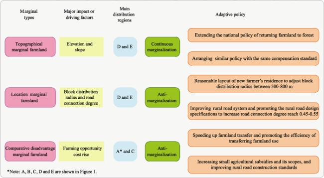
Based on SPOT-5 images, 1:1 million topographic maps, the maps of the returning farmland to forest project and the Chongqing forest project, social and economic statistics, etc., this paper identifies the features and factors influencing farmland marginalization. The results showed: (1) During 2002-2012, the rate of farmland marginalization was 16.18%, which was mainly found in the high areas of northern Qiyao mountains and the medium-altitude areas of southern Qiyao mountains. And this farmland marginalization will increase, associated with non-agriculturalization of rural labourers and aging of the remaining labourers. (2) Elevation, distance radius from villages and road connections had a great influence on farmland marginalization. Farmland marginalization rates showed an increasing trend with the increase of elevation, and 60.88% of the total farmland marginalization area is found at an altitude greater than 1000 m above sea level. The marginalization trend also increases with slope and distance from the distribution network. (3) Farmland area per labourer and the average age of farm labourers were major factors driving farmland marginalization. Farmland transfer and small agricultural machinery sets affect farmland marginalization with respect to management and productivity efficiency. (4) Farmland with “comparative- disadvantage-dominated marginalization” accounted for 55.32% of the total farmland marginalization area, followed by “location-dominated marginalization” (33.80%). (5) According to the specifics of each real situation, different policies are suggested to mitigate the marginalization. A “continuous marginalization” policy will encourage the return of farmland to forest in “terrain-dominated marginalization”. An “anti-marginalization” policy is suggested to create new rural accommodation and improve the rural road system to counteract “terrain-dominated marginalization”. And another “anti-marginalization” policy is planned to improve management and micro-mechanization for “comparative-disadvantage-dominated marginalization”. A new idea was developed to integrate high resolution remote sensing and statistical data with survey information to identify land marginalization and its driving forces in mountainous areas.

Cite this article

SHAO Jing’an , ZHANG Shichao , LI Xiubin . Farmland marginalization in the mountainous areas: Characteristics, influencing factors and policy implications[J]. Journal of Geographical Sciences, 2015 , 25(6) : 701 -722 . DOI: 10.1007/s11442-015-1197-4

1 Introduction

Farmland is often excluded from agricultural use in mountainous areas due to limiting factors such as undulating terrain, fragmented plots, and inconvenient transport links (Baumann et al., 2011; López-i-Gelats et al., 2011); we call this ‘farmland marginalization’. A large number of labourers have left rural areas (Liu and Li, 2005; Long et al., 2009), with the promotion of urbanization and the increasing opportunity cost of farming, against the background of co-development of urban and rural areas (Xin et al., 2011). High quality farmland is used more intensively under the influence of advances in technology, the transfer of farmland user rights, and moderate large-scale management (Aubry et al., 2012). Marginalization is driven by the joint effects of labour movement and more intensive land use. Undoubtedly, just like “forest transition” in developed countries, farmland marginalization also has a “win-win” effect in China (Woodhouse et al., 2005; Su et al., 2007; Li and Zhao, 2011). However, due to the high percentage of mountainous land in China (2/3 of the whole area), an appropriate balance must be established between food security and ecological protection.
Unfortunately, the literature presents a number of very common problems. First, the statistical analysis is relatively commonly used to illustrate the occurrence of farmland marginalization only by administrative regions (Robles et al., 2002; Renwick et al., 2013), so there is little information available on the spread of farmland marginalization conditions across regional administrative boundaries. Secondly, the qualitative description of the change from farmland to other types of land use pays more attention to characterizing the output from farmland marginalization (Mendola, 2008; Groom et al., 2010). The quantification of diagnostic criteria for the characterization of marginalization does not reflect the geographic character of the region (i.e., the site conditions). Thirdly, natural and human drivers of farmland marginalization are often confused in identifying the factors determining its occurrence (Silber and Wytrzens, 2006; Zaragozí et al., 2012; Kang et al., 2013), and no attempt is made to integrate the two types of factors. Finally, “an anti-marginalization” policy, involving an increase in the grain subsidy, the transfer of farmland contract rights, and so on, is actively promoted to protect farmland and ensure food safety (Giles, 2006; Wang et al., 2010; Zhao et al., 2012). At the same time there is no clear policy on “continuous marginalization” because of conflict with the farmland protection policy.
The overlay of high resolution images of the main crops in a non-growing season and previous 1:1 million standard topographic maps provided a convenient way to find the exact position of farmland marginalization. The average indices (e.g., elevation, slope, distance from village and road connections) were extracted at the block level, using the same scale of DEM, road and residential distribution maps. A logistic regression model between all farmland and the above indices provided an effective method to answer questions of farmland marginalization and related issues, and a stepwise regression model between farmland marginalization rate and socio-economic data was built at the village level. Thus, a new way was provided to quantitatively interpret the contribution of the factors driving the rate of farmland marginalization. The objective of this study was to identify the characteristics of farmland marginalization, to discover the main factors driving it, and to make adaptive “continuous marginalization” and “anti-marginalization” countermeasures.

2 Materials and methods

2.1 Study area

The study area, Shizhu County (107°59′-108°34′E, 29°39′-30°32′N), is located in the Wuling mountainous area, on the border of Chongqing City and Hubei Province (Figure 1). It covers an area of about 3012.24 km2. Two parallel mountain ranges running northeast-southwest cross the study area, with a relief pattern described as “two mountains, one groove and one plain”. The “two mountains” are Qiyao mountain and Fangdou mountain, “one groove” is the wide valley between the two mountains, and “one plain” is a small plain along the Yangtze River. The middle and low mountainous area accounts for 50% of the study area. The climate is the subtropical humid monsoon climate zone of the mountains of the surrounding Sichuan Basin, with an annual mean temperature of 16.5℃, and annual mean precipitation of 1103 mm. The main soil types include neutral and slightly acidic yellow soil, yellow-brown soil, purple soil and paddy soil. Vegetation consists of a subtropical evergreen broad-leaved forest and deciduous broad-leaved forest zone, with the forest coverage rate of 52.8% based on the results of 2nd-Class Survey Data from 2012.
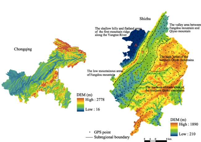
Figure 1 Location of Shizhou County in Chongqing and its topography
At the end of 2011 there were 32 townships, consisting of 229 villages and 134,000 households, involved in the study area, with a total of 544,500 people. Farmland, GDP and net income per capita was 0.13 ha, 19,396 yuan (calculated by permanent population), and 5981 yuan, respectively. According to “Key Ecological Function Protection and Construction Planning in Chongqing” (2011-2030), the study area belongs in a rocky desertification mountain key ecological recovery area. It represents an important biological gene pool and ecological barrier zone in the upper reaches of the Yangtze River.

2.2 Data collection

In 2011 SPOT-5 images at a 2.5-m resolution were provided by Chongqing Institute of Forestry Planning and Designing. 1:1 million topographic maps (2002), distribution maps of farmland returning to forest (2002-2006) and the Chongqing forest project (2008-2011) were collected from the Forestry Bureau of Shizhu County. 1:1 million village administrative boundaries, 1:1 million records from the second national land survey (2010), distribution maps of 1:1 million roads and residents were given by the Bureau of Land Resources and Housing Management of Shizhu County. DEM with a 30-m resolution came from the Western China Data Center. The authors of this paper sequentially surveyed the study area 12 times (a total of 50 survey days from June 30, 2011 to May 28, 2012) to collect field data.
In 2011 the population and socio-economic data for each village in 32 townships were obtained from the statistical yearbook of Shizhu County. Similarly, other data at the village level were collected from various reports of the relevant functional departments of the 32 townships. The area of contracted farmland, farmland area per capita, farmland transfer, etc., came from the land department of the townships concerned. The categories of farmers’ households and labourers, the output value of planting, the income from non-farm employment, etc., were derived from the Economic Development Office of the townships. The total population change, from agricultural to non-agricultural, was obtained from the township police stations. The number of live pigs and the value of the pig breeding industry were collected from the animal husbandry stations of the townships, and the number of small agricultural machinery sets was obtained from the township Government Offices. The authors also interviewed 120 farmers’ households three times (a total of 23 days of interviews from August 30, 2012 to November 25, 2012) to check and supplement parts of the data.

2.3 Data processing

The data on farmland and rural residents in 2002 were obtained from 1:1 million topographic maps. The information on farmland in 2011 was extracted using SPOT-5 images. In these images, the colour of the patches was uniformly light blue, light green or tea green, and the shape of the patches was generally regular and with clear boundaries, and they were categorized into the three groups referred to in this paper. The first was the returning farmland to forest project area (2002-2006), the second was distributed in the Chongqing forest project area (2008-2011), and the third was the farmland marginalization area.
The maps of the returning farmland to forest and the Chongqing forest projects were processed through format and projection transformation, and stacked in a standard topographic map with Xi'an 1980 coordinates. They were converted to .shp format after being vectored. When superimposing the maps the farmland returning to forest stands out.
The data (e.g., landscape photos, GPS coordinates, surveying record content, etc.), obtained through the field survey and interview, were imported into the above maps, validating the data set for farmland marginalization and at the same time incorporating the demographic and social and economic data collected at the village level.

2.4 Data analysis

(1) Determination of the overall pattern of farmland marginalization
As shown in Figure 2, farmland change between 2002 and 2011 were derived by superimposing farmland distribution maps from 2002 and 2011. The farmland marginalization map was obtained by subtracting the patches of farmland from the farmland returning to forest maps (2002-2006) and the Chongqing forest project maps (2008-2011), respectively.
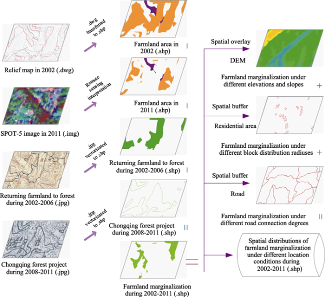
Figure 2 Treatment processes for obtaining farmland marginalization
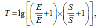
(2) Distribution of farmland marginalization under different site conditions
Site conditions involved terrain and location. Elevation and slope of the terrain were analysed primarily, and the relative distance away from the villages and road connections were also considered, due to their important influence on farmland marginalization.
Elevation and slope were classified into five grades, according to the results of “farmland classification and gradation in Shizhu County” (Table 1). Their different grading ranges were extracted using 3D analysis tools in ARCGIS, based on a 30-m resolution DEM.
The terrain position index was determined by calculating the heterogeneity of elevation and slope using the formula of Yu et al. (2001):
where T is terrain position index, and (E and ) and (S and ) are the elevation and slope at any point, and the mean elevation and slope of the region where this point is located, respectively. The division into five grades is shown in Table 1.
The relative distance away from the villages was measured using the Euclidean linear distance and the terrain position index, and classified into five grades (Table 1). The Euclidean linear distance of each farmland block away from the nearest villages was found, and then a terrain position index was used to revise the Euclidean linear distance. The corrected distance was regarded as the relative distribution radius of blocks of farmland away from the villages.
Table 1 The classification of elevation, slope, terrain position index and its correction coefficient, relative distribution radius from the villages, and degree of road connection
Factors Classification standard Factors Classification
standard
Factors Classification standard
Elevation (m) <450 Terrain position
index
<0.5 Relative distribution radius of block away from the villages (m) ≤150
450-750 0.5-1 150-300
750-1000 1-1.5 300-500
1000-1500 1.5-2 500-800
≥1500 ≥2 >800
Slope (°) <2 Correction coefficient of topographic position index 1 Degree of road connection ≤0.45
2-6 1.05 0.45-0.5
6-15 1.1 0.5-0.55
15-25 1.15 0.55-0.6
≥25 1.2 ≥0.6
Degree of road connection was measured using ARCGIS to extract the number of road network connections and nodes with the following formula
where γ is the degree of road connection, L is the number of actual connections in the road network, Lmax is the number of maximum possible connecting corridors in a road network, and V is the number of nodes. Correspondingly, the degree of influence of roads on farming convenience was also divided into five grades, based on “farmland classification and gradation in Shizhu County” (Table 1).
Farmland marginalization under different site conditions was obtained by overlaying the classification maps of the indices of site conditions (e.g., elevation, slope, relative distribution radius from villages, and degree of road connection) and the spatial distribution of farmland marginalization patterns (Figure 2).
(3) Relationship between causes and effects
According to the theory of land rent, land with poor site conditions often has a comparative disadvantage in obtaining rent. Market forces mean that such land is allocated to rural labour rather than non-agricultural industry with a higher income. The theory of comparative advantage dictates that successful marketization of the pig-breeding industry requires large-scale development, but poor site conditions prevent this. Also, on small blocks of land with poor site conditions the possibility of using small agricultural machinery is limited, so the costs of labour and infrastructure are higher. The relationship hypothesis between these different variables is shown in Tables 2 and 3.
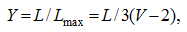
Table 2 Impact factors of farmland marginalization and their meanings
Factors Indicators Meanings Relationship
hypothesis
Terrain Elevation X11 The mean elevation where marginal farmland is located +
Slope X12 The mean slope where marginal farmland is located +
Location Relative distribution radius of block away from the villages X21 The mean actual distance of farmers’ blocks from their residence +
Road connection degree X22 The mean degree of convenience for farmers accessing their farmland of each block -
(4) Analysis of the factors impacting farmland marginalization
Terrain and location were selected as the explanatory variables due to their being closely related with land rent. The block was taken as the smallest analysis unit, and the meaning of the indicators is shown in Table 2.
The data of causes (explanatory variables) and effects (explained variables) were extracted at the block level. The explained variables (Y) were obtained through assigning the value 1 to marginal blocks and the value 0 to non-marginal blocks. The explanatory variables (X) were extracted by overlaying a farmland map showing assigned value and the classification maps of terrain and location.
The method of Logistic Regression Analysis was used to identify the relationship between Y and X, due to Y being one of the only two possibilities.
(5) Analysis of the driving factors of farmland marginalization
The socio-economic data had good spatial homogeneity at the village level. Moreover, the general trend between village administrative boundaries and DEM was consistent. Hence, the analysis of the driving factors of farmland marginalization had a strong comparability when selecting the village as the smallest unit.
The main driving factors of farmland marginalization fell into five categories, with 12 indicators (Table 3). Farmland area per labourer characterized the conditions of the labourers left behind who actually rely on the farmland area. Farmland transfer is an important way to optimize resource allocation. The average age of farm labourers and the rate of part-time labourers directly reflected the conditions of agricultural production, jointly determining the allocation of rural labourers and the rate of off-farm labour. The pig-breeding commercialization rate reflected the effects of the market on farmland use, and the rate of income from pig-breeding to total family income showed the degree of attention of the family to the market. The rate of off-farm income to total family income determined the allocation of family labour and farmland resources; a farmer’s degree of dependence on the farmland would be greatly reduced after transitioning from agricultural to non-agricultural employment. Small agricultural machinery sets substituting for human labour determined the possibility and farmland management on a moderate scale.
The rate of farmland marginalization at the village level was explained as variable (Y). It was extracted from the area of farmland marginalization for each village during 2002-2011, divided by the total area of contracted farmland in 2011. Explanatory variables (X) were measured by the meanings shown in Table 3.
Table 3 Driving factors of farmland marginalization and their meanings
Factors Indicators Meanings Relationship hypothesis
Farmland Farmland area per labour X11 Contracting farmland area divided by the sum of farm and concurrent labourers +
Rate of farmland transfer X12 Farmland transfer area divided by the area of contracting farmland -
Labour Rate of off-farm labour X21 Off-farm labourers divided by the sum of farm, concurrent and off-farm labourers +
Rate of concurrent labour X22 Concurrent labourers divided by the sum of farm, concurrent and off-farm labourers -
Average age of farm labour X23 Total age of farm labourers divided by the number of farm labourers +
Policy Rate of transferring from agricultural to non-agricultural population X31 Transferring from agricultural to non-agricultural population divided by total population +
Small agricultural machinery
sets X32
How many small agricultural machinery sets were bought by farmers -
Market Planting commercialization rate X41 Income obtained by selling planting productions divided by planting output -
Pig-breeding commercialization
rate X42
Income obtained by selling pig productions divided by pig output -
Income Rate of planting income X51 Planting income divided by family total income -
Rate of pig-breeding income X52 Pig-breeding income divided by family total income -
Rate of off-farm income X53 Off-farm income divided by family total income +
The multivariate regression model was built using Stepwise regression, and the order of importance and function as a direction of the driving factors were quantified by it.

3 Results and discussion

3.1 Overall characteristics of farmland marginalization

The proportion of the farmland marginalization area divided by the farmland reduction area accounted for more than 50% in the past ten years. The area of farmland marginalization during 2002-2011 was 11,575.87 ha, and the rate of farmland marginalization was 16.18% (Table 4). Referring to the area of farmland in 2002, the farmland marginalization area, which accounted for 50.61% of the total decrease area, was greater than the total area involved in the return of farmland to forest and in the Chongqing forest project changing forest to farmland. In other words, this result indicates that returning farmland to forest and the Chongqing forest project have the opportunity for further expansion.
The decrease of dry farmland was the main component of farmland marginalization over the past ten years. The area of dry farmland marginalization was 9722.22 ha during 2002-2011 (Table 4), accounting for 83.99% of the total farmland marginalization area, while the area of paddy marginalization accounted for only 16.01%. The area of dry farmland marginalization accounted for 46.44% of the decrease in the area of dry farmland, slightly lower than the scale of dry farmland returned to forest under the process of returning farmland to forest. The area of dry farmland marginalization was significantly higher than that of paddy marginalization. This result showed that the possibility of paddy marginalization was lower, due to the paddy being relatively fertile. The possibility of dry farmland marginalization was higher, due to a large number of young migrant rural labourers.
Table 4 Area and its rate of farmland marginalization during 2002-2011, and implementation scale of returning farmland to forest during 2002-2006 and Chongqing forest project during 2008-2011 (ha and %)
Land types Farmland in 2002 Actual
farmland use in 2011
Contracting farmland in 2011 Farmland decrease during 2002-2011 Returning farmland to forest
during 2002-2006
Chongqing forest project during 2008-2011 Farmland marginalization
during 2002-2011
Area Rate of area to actual
farmland use in 2011
Dryland 52800.44 31865.34 41587.56 20935.10 10618.37 594.51 9722.22 23.38
Paddy 30029.56 28090.74 29944.39 1938.82 - 85.17 1853.65 6.19
Total 82830.00 59956.08 71531.95 22873.92 10618.37 679.68 11575.87 16.18
The spatial distribution of farmland marginalization presented significant heterogeneity (Table 5 and Figure 3). The rate of farmland marginalization was the highest in the high mountainous areas of northern Qiyao mountain, a rate of 42.53%. Next were the middle mountainous areas of southern Qiyao mountain and the low mountainous areas of Fangdou mountain, accounting for 17.95% and 16.95%, respectively. 9.19% of the total farmland area was in the high mountainous areas of northern Qiyao mountain, where the proportion of the area of farmland marginalization to its total farmland area was 24.14%. Accordingly, the difference between the latter and the former only was 2.97 percentage points in the middle mountainous areas of southern Qiyao mountain. Opposite results occurred in the shallow hilly and flatland areas of the first mountain ridge along the Yangtze River, and the valley area between Fangdou mountain and Qiyao mountain.
Table 5 Area and its rate of farmland marginalization during 2002-2011, and implementation scale of the returning farmland to forest project during 2002-2006 and Chongqing forest project during 2008-2011 in different regions (ha and %)
Subregion Land
types
Actual
farmland use
in 2011
Contracting farmland
in 2011
Returning
farmland to
forest during 2002-2006
Chongqing
forest
project during 2008-2011
Farmland marginalization
during 2002-2011
Area Rate of its area to contracting
farmland in 2011
A* Dry farmland 4497.87 5177.74 2406.82 127.14 679.87 13.13
Paddy 3603.62 3801.06 - 30.07 197.44 5.19
Subtotal 8101.49 8978.80 2406.82 157.21 877.31 9.77
B Dry farmland 2130.72 2742.20 497.59 21.01 611.48 22.30
Paddy 1222.45 1295.48 - 1.29 73.03 5.64
Subtotal 3353.17 4037.68 497.59 22.30 684.51 16.95
C Dry farmland 13020.34 15618.05 5083.39 106.03 2597.71 16.63
Paddy 15753.56 16885.02 - 39.35 1131.46 6.70
Subtotal 28773.90 32503.07 5083.39 145.38 3729.17 11.47
D Dry farmland 2215.62 4894.33 159.86 8.33 2678.71 54.73
Paddy 1560.44 1676.17 - - 115.73 6.90
Subtotal 3776.06 6570.50 159.86 8.33 2794.44 42.53
E Dry farmland 10000.79 13155.24 2470.71 332.00 3154.45 23.98
Paddy 5950.67 6286.66 - 14.46 335.99 5.34
Subtotal 15951.46 19441.90 2470.71 346.46 3490.44 17.95

*Note:A, B, C, D and E are shown in Figure 1.

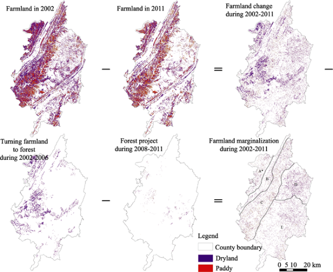
Figure 3 Spatial distributions of farmland decrease during 2002-2011, returning farmland to forest during 2002-2006, Chongqing forest project during 2008-2011, and farmland marginalization during 2002-2011
The spatial distribution of dry farmland and paddy marginalization rates presented a reverse trend. As shown in Table 5 and Figure 3, regional differences in the dry farmland marginalization rate were very significant, while the spatial heterogeneity of paddy marginalization rate was relatively small, with a range of 5.19%-6.90%. The rate of dry farmland marginalization was most prominent in the Fangdou mountain and the Qiyao mountainous areas, accounting for 54.73% in the high mountainous areas of northern Qiyao mountain. However, it only accounted for 13.13% in the shallow hilly and flatland areas of the first mountain ridge along the Yangtze River.
The spatial distribution of the farmland marginalization rate and the returning farmland to forest and Chongqing forest projects showed similar patterns (Table 5 and Figure 3). The proportion of the total area of the returning farmland to forest project (2002-2006) and the Chongqing forest project (2008-2011) to the total farmland area (2002) was larger, and the rate of farmland marginalization during 2002-2011 was lower. In the high mountainous areas of northern Qiyao mountain, the former was only 2.50%, while the latter reached as high as 42.53%. The opposite result occurred in the shallow hilly and flatland areas of the first mountain ridge along the Yangtze River.

3.2 Distributions of farmland marginalization under different site conditions

As shown in Table 6, farmland marginalization showed a significantly increasing trend with elevation. The negative correlation between elevation and farmland can easily be seen. Lower elevations had a lower farmland marginalization rate, with only 9.25% at elevations ≤450 m, with the rate of marginalization rising at higher elevations, up to 47.41%, although only 5.93% of the total farmland area was distributed in the high elevation zone.
The distribution of farmland marginalization in association with slope was similar to that with elevation (Table 6). The rate of farmland marginalization was the lowest at a slope of 6°-15° (14.09%), while it was the highest when the slope ≥25° (up to 22.53%). It was slightly lower (15.25%) than the average level for the 76.38% of total farmland area with a slope ≤15°. The 17.60% of the total farmland area with a slope between 15°-25° was 1.9 percentage points higher than the average. The 6.02% of the total farmland area with a slope ≥25° was 1.39 times the average level, and was 1.48 times that at a slope ≤15°.
Table 6 Area and its rate of farmland marginalization during 2002-2011, and the actual farmland use and contracting farmland in 2011 under different site conditions (ha and %)
Site
conditions
Index
classification
Actual
farmland use
in 2011
Contracting
farmland
in 2011
Farmland marginalization
during 2002-2011
Area Rate of its area to
contracting farmland in 2011
Elevation (m) <450 7232.07 7969.27 737.20 9.25
450-750 11931.37 13449.52 1518.15 11.29
750-1000 16188.83 18462.42 2273.59 12.31
1000-1500 22374.32 27411.36 5037.04 18.38
≥1500 2229.49 4239.38 2009.89 47.41
Slope (°) <2 18243.78 21508.12 3264.34 15.18
2-6 9277.01 11052.81 1775.80 16.07
6-15 18782.45 22071.69 3289.24 14.90
15-25 10314.96 12590.94 2275.98 18.08
≥25 3337.88 4308.39 970.51 22.53
Block distribution radius (m) ≤150 3166.94 3511.39 344.45 9.81
150-300 10256.62 11464.69 1208.07 10.54
300-500 13286.95 14941.28 1654.33 11.07
500-800 15682.78 18305.96 2623.18 14.33
≥800 17562.79 23308.63 5745.84 24.65
Road connection degree ≤0.45 31491.93 39423.52 7931.59 20.12
0.45-0.5 17133.62 19447.36 2313.74 11.90
0.5-0.55 8828.45 9932.00 1103.55 11.11
0.55-0.6 2097.27 2297.78 200.51 8.73
≥0.6 404.81 431.29 26.48 6.14

*Note: A, B, C, D and E are shown in Figure 1.

Farmland marginalization increased along with the relative distribution radius of farmland blocks away from the villages. The rate of farmland marginalization presented no significant difference when the distribution radius was ≤500 m, and at 14.33% was still lower than the overall level at a distribution radius between 500-800 m. However, it was significantly increased at a distribution radius ≥800 m, being 1.52 times the overall level. Therefore we considered that the largest farming radius was currently 800 m in the study area. Only 6.02% of the total farmland area was concentrated in a distribution radius >500 m.
Farmland marginalization appeared to decrease with degree of road connection. The rate of farmland marginalization was 1.52 times the overall level at a road connection degree ≤0.45, while it was lower than the overall level at a degree of road connection between 0.45-0.55, and was 48.58% the overall level, when road connection degree increased to ≥0.55. It was as high as 68.52% at a road connection degree ≤0.45, which accounted for 76.38% of the total farmland area. However, it was 29.52%, when the road connection degree was between 0.45 and 0.55. Thus, we considered that a road connection degree between 0.45 and 0.55 was very relevant.

3.3 Factors impacting farmland marginalization

A study on logistic regression model between farmland marginalization occurring or not and main terrain and location factors was carried out according to the formula
After simplification,
=Y=0.797+0.052 X12+0.117X21+0.095X11-0.579X22.
As shown in Table 7, the fitting results were very good, with a prediction accuracy of 72.9%. A positive coefficient showed that the explained variable was equal to 1 with a greater probability, while a negative coefficient indicated that the explained variable was equal to 1 with a smaller probability. The road connection degree had the greatest impact on farmland marginalization, followed by the relative distribution radius of blocks away from the villages. Moreover, the block distribution radius, elevation and slope showed a positive effect, while the impact of road connection degree was the opposite.
Table 7 Logistic regression between farmland marginalization and its impact factors
Variables B S.E, Wals df Sig. Exp (B)
X12 0.052 0.011 23.564 1 0.000 1.054
X21 0.117 0.013 82.853 1 0.000 1.124
X11 0.095 0.012 60.906 1 0.000 0.910
X22 -0.597 0.013 2047.090 1 0.000 0.550
Constants 0.797 0.013 3512.485 1 0.000 2.219
Cox & Snell R Square 0.359
Nagelkerke R Square 0.380
-2 Log likelihood 51751.333
Prediction accuracy 72.9%
The relative distribution radius of blocks away from the villages was the most important of all positive impact factors on farmland marginalization. The farming radius decreased gradually, due to rural labour migration and residents who abandoned driving altogether. Farmland outside of the farming radius was easily marginalized. The result was consistent with the hypothesis of the generalization law of the function of block distribution radius to the differential land rent I. The number of villages was reduced by 60.43% during 2002-2011 in the study area, and the size of villages decreased by 14.04%.
Elevation ranked second of all positive impact factors on farmland marginalization. The high altitude mountainous area usually took the lead in becoming marginal, because of undulating terrain, inconvenient transport, high cost facilities, etc. Moreover, under the laws of market forces, labourers preferentially selected non-agricultural industries with a higher income, and infrastructure went first to relatively flat areas. This result is consistent with the hypothesis of the generalization law of the function of elevation relative to the differential land rent I. As shown in Table 6, 60.88% of the farmland marginalization area appeared in the middle mountain areas at elevations of more than 1000 m.
Slope was the third ranking of all positive impact factors on farmland marginalization. When it was greater, farming convenience was reduced, farmland was easily marginalized, due to the obvious comparative disadvantage. This result is consistent with the hypothesis of the generalization law of the function of slope relative to the differential land rent I. The rate of farmland marginalization did not present significant differences at slopes <15° (Table 6). Hence, we considered that the slope <15° was a relatively appropriate planting zone.
The negative influence of road connection degree on farmland marginalization can be seen. When road connection degree was higher, farming accessibility was better. Under such an environment, the farming radius was larger, and farmland was not easily marginalized. This result is consistent with the hypothesis of the generalization law of the function of road connection degree relative to the differential land rent I. Some rural roads in the study area were abandoned during 2002-2011, because of a large amount of labour migration. In addition, some out-of-the-way roads also were abandoned due to farmland consolidation and new rural residential construction. The number of rural roads saw a reduction of 43.57% during 2002-2011 in the study area, with the mileage of rural roads decreasing by 23.46%. The number of rural roads was reduced, their mileage decreased, and the accessibility of the roads deteriorated, so the farmland that the original roads accessed was marginalized.

3.4 Driving factors of farmland marginalization

A stepwise regression model between the farmland marginalization rate and driving factors was built, with the following formula
lnY=-3.745+0.557lnX11+1.459 lnX23-0.172lnX12-0.129lnX32+0.150lnX21.
Successfully simulated results were obtained with this equation, with an absolute value of t>2 (R2=0.891), as shown in Table 8. Farmland area per labourer had the greatest effect on farmland marginalization, followed by the average age of the farm labourer, the rate of farmland transfer and the number of small agricultural machinery sets. Farmland area per labourer, the average age of the farm labourer, and the rate of off-farm labour showed positive effects on farmland marginalization, while the impacts of the rate of farmland transfer and the number of small agricultural machinery sets was negative.
Table 8 Stepwise regression between farmland marginalization and its driving factors
Variables Not standardized coefficient Standard
coefficient
t Sig. R2 F
B Standard error
(Constant) -3.745 0.700 - -5.353 0.000 0.891 361.12
lnX11 0.557 0.069 0.445 8.058 0.000
lnX23 1.459 0.391 0.177 3.732 0.000
lnX12 -0.172 0.058 -0.147 -2.967 0.003
lnX32 -0.129 0.042 -0.152 -3.098 0.002
lnX21 0.150 0.055 0.091 2.728 0.007
The impact of farmland area per labourer on farmland marginalization was very significant, and there was a positive correlation between them. The allocation preference of labour resources took the lead in selecting non-agricultural industry with a better income. Thus, the number of remaining labourers who were engaged in agricultural production was generally reduced. This result is consistent with the hypothesis of the basic laws of market allocation of resources. The rate of off-farm labourers in the study area was up by 46.54% in 2011 (Figure 4a). Farmland area per labourer increased, basically doubling that of previous rural labourers going out to make money. Certainly, the most direct consequence of the increase of farmland area per labourer was that some of the farmland was not cultivated, or could not be effectively utilized, especially if the farmland had bad site conditions. In addition, the remaining labourers were not fully engaged in agricultural production. The rate of concurrent labour in the study area was as high as 19.71% in 2011.
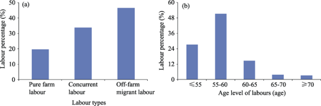
Figure 4 The allocation patterns of labour resource
The average age of farm labourers had similar driving effects on farmland marginalization, compared with farmland area per labourer. The aging of farming labourers leads to the farming radius being reduced greatly. Blocks were inevitably marginalized when their location was more than the farming radius. This result is also consistent with the hypothesis of the basic laws of market allocating resources. When young rural labourers transferred to non-agricultural industries, the labourer age structure changed significantly. The remaining labourer average age was over 50, and even some of the workforce >70 years old was still in farming. As shown in Figure 4b, the age of farming labourers was mainly between 56-60 years old in the study area, accounting for 51.16% of total. However, the farming labourers ≤55 years old only accounted for 27.29%, and farming labourers >70 years of age represented only 3.22%.
Farmland transfer had a clearly inverse effect on farmland marginalization. The scale of the blocks was increased, due to farmland transfer, small agricultural machinery could be used easily. The cost of supporting infrastructure construction was kept down, and its efficient use was improved. The comparative advantage of this kind of farming was significant, and farmland marginalization did not often occur. This result is consistent with the hypothesis that resource agglomeration rules pursue a scale effect. The rate of farmland transfer in the study area was up to 25.23% in 2011 (Figure 5a). Moreover, the number of villages with a farmland transfer rate ≥20.0% accounted for 81.66% of the total.
The relation of small agricultural machinery sets to farmland marginalization was also inverse. When the number of small agricultural machinery sets on 100 ha farmland increased, the probability of farmland marginalization declined. This result is consistent with the general hypothesis that machines replace human labour. In the study area, 100 ha farmland had an average of 19.8 sets of small agricultural machinery in 2011. The rate of farmland marginalization reduced from 28.27% to 8.09%, with a corresponding change in the number of small agricultural machinery from ≤10 sets to ≥30 sets per 100 ha, respectively (Figure 5b). Thus, the chance of farmland marginalization occurring was decreased when semi-mechanized operation, with small machinery replacing human labour, was implemented at the local scale.
Figure 5 Distributions of farmland transfer (a) and relationships between small mechanical sets per 100 hectares and farmland marginalization rate (b)
The impact of the rate of off-farm labourers on farmland marginalization was adverse. As shown in Figure 6a, rising non-farm labourer wages resulted in an increase of farmland area per labourer and in the average age of farm labourers. Consequently, farming radius was reduced, and the ability of labourers to develop the capacity of the farmland decreased. This result is also consistent with the hypothesis that the market allocates resources. The rate of off-farm labourers in the study area was 46.54% in 2011. Moreover, it grew from 28.34% to 65.82%, associated with the increase in the rate of farmland marginalization from 9.62% to 31.38% (Figure 6b). Young rural labourers were the first to be attracted to non-agricultural industries, with an obvious comparative advantage, and the appeal to labourers of agriculture was more limited.
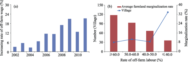
Figure 6 Increasing rate of off-farm wage (a) and relationships between rate of off-farm labour and farmland marginalization rate (b)
According to the above theoretical hypothesis, the driving force of the rate of transfer from an agricultural to a non-agricultural population is obvious, although this was not apparent based on a significant test in the Stepwise regression model. Population transfer from agriculture to non-agriculture was up to 56,101 between 2010 and 2011, but the effects of this on farmland marginalization were smaller due to it involving three groups. The first group (accounting for 47.62%) was the rural labourers who migrated perennially to work, and most of their contracted farmland had already been transferred to others. The second group (accounting for 5.17%) included the village cadres, who did not leave the land and were still engaged in agricultural production. The third group (accounting for 47.21%) was the old and the sick, who were unable to work.
As shown in Figure 7, the rate of off-farm (planting) income among villages was not significantly different in 2011. Off-farm income was the main source of family income, and on average accounted for 43.50% of family total income. The number of villages, with an anomaly variation rate of off-farm income between ±5%, was up to 72.05% of total villages.
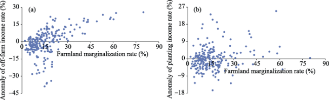
Figure 7 Relationships between anomaly of off-farm income rate (a) and planting income rate (b) and farmland marginalization rate
Then planting income (accounting for 19.42%) gradually dropped out the dominant position which supported family life. The number of villages, with the anomaly variation of rate of planting income between ± 5%, was up to 81.36% of total villages. Thus, the effects of rate of off-farm (planting) income on farmland marginalization rate did not occur significantly.
The differences in the rate of pig-breeding commercialization and rate of concurrent labour among villages were both very significant in 2011. The number of villages, with their anomaly variation rate between ±5%, accordingly was up to 69.00% and 86.03%, respecttively (Figure 8). The study area belonged to the typically traditional “grain-pig” agricultural region. However, pig breeding was mainly concentrated in a few large households, associated with the development of a large-scale breeding district (Figure 9a). Forage supply for large breeding households mainly came from designated markets outside the study area, or from the agglomeration of dispersed planting farmers’ households inside it.
When the rate of concurrent labour was larger, the probability of farmland marginalization occurring was smaller, and the number of villages with non-agricultural income greater than planting income accounted for 25.11% (Figure 9b). Non-agricultural industry was the main work of concurrent labourers, who only cultivated farmland that was not marginalized. Concurrent labour only participated in a limited range of non-agricultural production in these villages, where non-agricultural income at home was below 60% of planting income. But the differences in rate of off-farm labour, corresponding to the rate of concurrent labour, were not significant, at ±5%. This resulted in the impact of concurrent labour on farmland marginalization not being significant.
Figure 8 Relationships between anomaly of breeding commercialization rate (a) and concurrent labour rate (b) and farmland marginalization rate
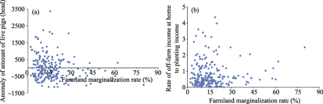
Figure 9 Relationships between anomaly of amount of live pigs (a) and rate of off-farm income at home to planting income (b) and farmland marginalization rate

3.5 Policy implications of farmland marginalization

The area of farmland with a “comparative-disadvantage-dominated marginalization” was 6403.84 ha, accounting for 55.32% of the total farmland marginalization area, followed by “location-dominated marginalization” (33.80%), while the lowest was “terrain-dominated marginalization” (Table 9). The spatial distribution of “comparative-disadvantage-
dominated marginalization” was most widespread in the shallow hilly and flatland areas of the first mountain ridge along the Yangtze River and in the valley area between Fangdou mountain and Qiyao mountain. “Location-dominated marginalization” and “terrain-
dominated marginalization” were mainly found in the high mountainous areas of northern Qiyao mountain and the middle mountainous areas of southern Qiyao mountain. The above results can be seen in Figure 10.
Steep slope farmland (slope≥25°) should belong to the category of farmland returning to forest. High mountainous areas (elevation ≥1500 m and slope between 15° and 25°) be-
came the first marginal zone, due to their higher elevation, steeper slope and greater overlap with forested areas. Poor terrain was the main limiting factor. Farmland marginalization was “terrain-dominated” because it was mainly affected by terrain conditions.
Table 9 Area of farmland marginalization types and their distributions in different regions
Subregion Terrain-dominated
marginalization
Location-dominated marginalization Comparative-disadvantage-dominated marginalization
Area (ha) Rate (%) Area (ha) Rate (%) Area (ha) Rate (%)
A* 13.39 1.06** 67.55 1.73 796.37 12.44
B 58.55 4.65 259.29 6.63 366.67 5.73
C 185.79 14.75 290.37 7.42 3253.01 50.80
D 299.28 23.76 1690.46 43.21 804.7 12.57
E 702.74 55.78 1604.61 41.01 1183.09 18.47

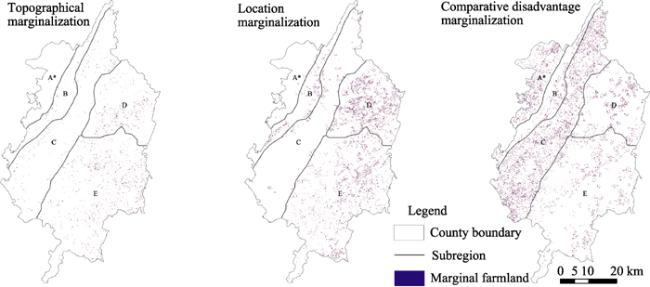
*Note: A, B, C, D and E are shown in Figure 1.

**It was the rate of the area of each farmland marginalization type under different regions to the total area of corresponding marginalization type in the study site.

Figure 10 Regional distributions of different farmland marginalization types

*Note: A, B, C, D and E are shown in Figure 1.

For the remaining elevations and slopes, the relative distribution radius of farmland blocks away from the villages was ≥800 m, and road connection degree was ≤0.45. The remaining labourers found it difficult to successfully produce agricultural materials on these blocks and transport them home at harvest time. Here “location-dominated marginalization” occurred naturally, resulting from the distribution location of block and village. As shown in Figure 10, this mainly occurred in the Qiyao and Fangdou mountainous areas, where the undulating terrain was relatively severe, the residential distribution was more dispersed, and the support of the road infrastructure was poor.
The increase of farming opportunity costs caused large numbers of young rural labourers to move to non-agricultural industries, resulting in “comparative-disadvantage-dominated marginalization”, with the widest distribution in the shallow hilly and flatland area of the first mountain ridge along the Yangtze River, and the valley area between Fangdou mountain and Qiyao mountain (Figure 10). Here, terrain and location were no longer the main conditions to restrict farming, but rather the increase of farming opportunity cost was the primary reason, with the result that a large number of young labourers moved to non-agricultural industries. Consequently, farmland area per labourer greatly increased, and the remaining labourers could only farmland closer to their home; more distant farmland tended to be marginalized.
Appropriate policies were developed (Figure 11), considering the main reasons for the occurrence of different marginal types. Farmland with “terrain-dominated marginalization” still did not have the comparative advantage for cultivation, because of its special site conditions (slope≥25° and elevation≥1500 m), even if the slope was reduced and location conditions were enhanced to fulfill the requirements for farming. Hence, the adaptive policy of “continuous marginalization” was most appropriate. The similar policy of continually extending returning farmland to forest nationwide was designed, and this allowed marginalized farmland to be preserved in its marginalized state forever, with the help of the farmers themselves in the “marginalization” trend. The compensation standard and length of service of the policy was not less than the regulations for returning farmland to forest.
Figure 11 Marginal types, major impact or driving factors, main distribution regions, and adaptive policy
The relative distribution radius of farmland blocks ≥800 m from the villages and the degree of road connection of ≤0.45 were the main restrictive factors affecting farming for “location-dominated marginalization”. Moreover, farmland with “location-dominated marginalization” will continue to expand in the future, being associated with the further transfer of rural labourers and the aging of the labourers left behind. An “anti-marginalization” policy was the result, due to it not being limited by slope and elevation.
New rural accommodation was constructed so that the distance to contracted farmland was between 500 and 800 m, following the principle of “overall dispersion, local concentration”. In the study area, the main reason that 78.32% of the farmers were unwilling to move to the central village was that it was too far away from their contracted farmland.
The rural road system was improved to regulate the degree of road connection. The rural road network density (85.17 km/100km2) in the study area was lower than that in Chongqing in 2011 (123.2 km/100km2). Moreover, 75.41% of directly-servicing agricultural production roads were earthen or gravel roads. Their width specification was generally below 0.8 m, similar to that of production roads. Tractor ploughing roads, with a width specification above 3.0 m, were mainly distributed in the farmland concentrated area. Therefore, degree of road connection was increased to 0.45-0.55 through improving the rural road system, with the help of land consolidation, high standard basic farmland construction, and new countryside construction.
For farmland with “comparative-disadvantage-dominated marginalization”, the farmland area per labourer and the average age of farm labourers could not be reduced by mandatory measures to limit the migration of young labourers, which would be unacceptable as well as being in conflict with the strategic demand to speeding up urbanization. Hence, appropriate guide policies were arranged, aiming at accelerating farmland transfer and small agricultural machinery promotion. That is, farmland beyond the capability of the labourers was transferred, and small agricultural machinery management, on a moderate scale, was implemented, with the support of land consolidation, roads, and water conservancy facilities.
In the farmland transfer area, the dominant characteristic regional agricultural industry was determined, and land consolidation, high-standard basic farmland construction, etc., primarily guided by the government, were vigorously carried out. At the same time, the financing channels for agricultural production were broadened. Thus, related resources were integrated, relying on transferred farmland, and the path of “comparative-disadvantage- ominated marginalization” was cut off.
For the promotion of small agricultural machinery, famers’ purchase subsidies needed to be increased. Moreover, subsidized servicing, repair, and maintenance after purchase also needed to be gradually phased in. Thus, small agricultural machinery was able to provide the full or partial replacement of agricultural labourers, and farmland was not marginalized because of the increase of farmland area per labourer, the loss of young rural labourers or the reduction of farming radius.

4 Conclusions

(1) The area of farmland marginalization during 2002-2011 was 11,575.87 ha, and the rate of farmland marginalization was 16.18% in the study area. It was mainly distributed in the high mountainous areas of northern Qiyao mountain and the middle mountainous areas of southern Qiyao mountain. More importantly, farmland marginalization will continue to increase in the study area, associated with the non-agriculturalization of rural labourers and the aging of the remaining labourers.
(2) At the “block” level, the relative distribution radius of blocks away from the villages and at elevation had a strong tendency to lead to farmland marginalization. Moreover, this paper found that the largest farming radius was 800 m, and a road connection degree between 0.45 and 0.55 was very appropriate. At the “village” level, the positive driving role of farmland area per labourer, average age of farm labourer and rate of off-farm labourers on farmland marginalization was discovered, whereas an opposite result was found for the effects of rate of farmland transfer and use of small agricultural machinery sets.
(3) The area of farmland with “comparative-disadvantage-dominated marginalization” was 6403.84 ha, which accounted for 55.32% of the total farmland marginalization area, followed by “location-dominated marginalization” (33.80%), while the lowest was “terrain-dominated marginalization”.
(4) A “continuous marginalization” policy, being similar to returning farmland to forests, was implemented to maintain the state of “terrain-dominated marginalization”. However, an “anti-marginalization” policy involving new rural accommodation and improving the rural road system was suggested for “location-dominated marginalization”; while an “anti-marginalization” policy to improve the utilization of transferred farmland and the new increasing after-sale service of small agricultural machines was proposed for “comparative-disadvantage-dominated marginalization”.
This paper used the combination of high resolution remote sensing images, statistical data and farmer’s interview data, in order to extract farmland marginalization and analyse its driving factors. Moreover, hierarchical interpretation for farmland marginalization was carried out at the “block” and “village” scale. On this basis, farmland marginalization was divided into three categories, i.e., “terrain-dominated marginalization”, “location-dominated marginalization” and “comparative-disadvantage-dominated marginalization”.
However, quantitative prediction of the future development trends of farmland marginalization could not be carried out because the social and economic statistical data used in this paper are “cross sectional data”. A model mechanism would be needed to achieve the above goals, based on time series data. Moreover, the results from some of the variables in this paper contradicted existing findings. In particular, the analysis of rate of transfer from an agricultural to a non-agricultural population, the rate of off-farm income, breeding commercialization rate, etc., contradicted current knowledge (Ding et al., 2009; Zhao et al., 2012). A detailed analysis found that the reasons for the above contradictions occurring were mainly found in three aspects. For the transfer from an agricultural to a non-agricultural population, the relevant population was not the moving farm labourers, but the remaining farming labourers. Off-farm income was the main source of family income, and the difference of rate of off-farm income was not significant among the different villages. For the breeding industry, the volume of scattered breeding farmers was smaller, and the forage supply in the large-scale breeding district mainly came from designated markets outside the study area, or the agglomeration of dispersed planting farmers’ households inside the study area. Moreover, the difference of breeding commercialization rates was not significant between the different villages. Hence, the effects of the above three aspects on farmland marginalization were not significant.

The authors have declared that no competing interests exist.

1
Aubry C, Ramamonjisoa J, Dabat M Het al., 2012. Urban agriculture and land use in cities: An approach with the multi-functionality and sustainability concepts in the case of Antananarivo (Madagascar).Land Use Policy, 29(2): 429-439.

2
Baumann M, Kuemmerle T, Elbakidze Met al., 2011. Patterns and drivers of post-socialist farmland abandonment in Western Ukraine.Land Use Policy, 28(3): 552-562.

3
Ding Guangping, Liu Chengwu, Huang Limin, 2009. A theoretical analysis and empirical research of marginalization of agricultural land in hilly-mountainous area under farmer-benefiting policy: A case study of Tongcheng County in Hubei Province.Geographical Research, 28(1): 109-117. (in Chinese)

4
Giles J, 2006. Is life more risky in the open? Household risk-coping and the opening of China’s labor markets.Journal of Development Economics, 81: 25-60.

5
Groom B, Grosjean P, Kontoleon Aet al., 2010. Relaxing rural constraints: A ‘win-win’ policy for poverty and environment in China?Oxford Economic Papers, 62: 132-156.

6
Kang S, Post W, Wang Det al., 2013. Hierarchical marginal land assessment for land use planning.Land Use Policy, 30(1): 106-113.

7
Li Xiubin, Zhao Yuluan, 2011. Forest transition, agricultural land marginalization and ecological restoration.China Population, Resources and Environment, 21(10): 91-95. (in Chinese)

8
Liu Chengwu, Li Xiubin, 2005. The character and diagnostic criterion for marginalization of the arable land.Progress in Geography, 24(2): 106-113. (in Chinese)

9
Long Hualou, Zou Jian, Liu Yansui, 2009. Differentiation of rural development driven by industrialization and urbanization in eastern coastal China.Habitat International, 33(4): 454-462.

10
López-i-Gelats F, José Milán M, Bartolomé J, 2011. Is farming enough in mountain areas? Farm diversification in the Pyrenees.Land Use Policy, 28(4): 783-791.

11
Mendola M, 2008. Migration and technological change in rural households: Complements or substitutes?Journal of Development Economics, 85: 150-175.

12
Renwick A, Jansson T, Verburg P Het al., 2013. Policy reform and agricultural land abandonment in the EU.Land Use Policy, 30(1): 446-457.

13
Robles A B, Allegretti L I, Passera C B, 2002. Coronilla juncea is both a nutritive fodder shrub and useful in the rehabilitation of abandoned Mediterranean marginal farmland.Journal of Arid Environments, 50(3): 381-392.

14
Silber R, Wytrzens H K, 2006. Modelling the probability of land abandonment at parcel level.Jahrbuch der Österreichischen Gesellschaft für Agrarökonomie, 15: 55-63.

15
Su Yongzhong, Wang Fang, Zhang Zhihuiet al., 2007. Soil properties and characteristics of soil aggregate in marginal farmlands of oasis in the middle of Hexi Corridor Region, Northwest China.Agricultural Sciences in China, 6(6): 706-714.

16
Wang Hui, Tao Ran, Wang Lanlanet al., 2010. Farmland preservation and land development rights trading in Zhejiang, China.Habitat International, 34(4): 454-463.

17
Woodhouse S P, Good J E G, Lovett A Aet al., 2005. Effects of land-use and agricultural management on birds of marginal farmland: A case study in the Llŷn peninsula, Wales.Agriculture, Ecosystems & Environment, 107(4): 331-340.

18
Xin Liangjie, Li Xiubin, Tan Minghonget al., 2011. The rise of ordinary labor wage and its effect on agricultural land use in present China.Geographical Research, 30(8): 1391-1400. (in Chinese)

19
Yu Hong, Zeng Hui, Jiang Ziying, 2001. Study on distribution characteristics of landscape elements along the terrain gradient.Scientia Geographica Sinica, 21(1): 64-69. (in Chinese)

20
Zaragozí B, Rabasa A, Rodríguez-Sala J Jet al., 2012. Modelling farmland abandonment: A study combining GIS and data mining techniques. Agriculture, Ecosystems & Environment, 155(15): 124-132.

21
Zhao Yuluan, Li Xiubin, Xin Liangjieet al., 2012. Driving forces of “poplar expansion and cropland shrinkage” in the North China Plain: A case study of Wen’an County, Hebei Province.Geographical Research, 31(2): 323-333. (in Chinese)

Outlines

/