Orginal Article

The change in population density from 2000 to 2010 and its influencing factors in China at the county scale

  • WANG Lu , 1, 2 ,
  • FENG Zhiming , 1, * ,
  • YANG Yanzhao , 1, *
Expand
  • 1. Institute of Geographic Sciences and Natural Resources Research, CAS, Beijing 100101, China
  • 2. University of Chinese Academy of Sciences, Beijing 100049, China

*Corresponding author: Feng Zhiming, PhD and Professor, E-mail:;Yang Yanzhao, PhD, E-mail:

Author: Wang Lu (1986-), specialized in Population, Resource and Environmental Economics. E-mail:

Received date: 2014-02-22

  Accepted date: 2014-03-20

  Online published: 2015-04-15

Supported by

Key Project of National Natural Science Foundation of China, No.41430861

Foundation of Bureau of Floating Population, National Health and Family Planning Commission of China, No.201011

Copyright

Journal of Geographical Sciences, All Rights Reserved

Abstract

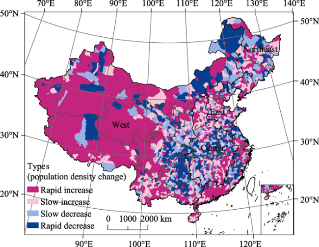
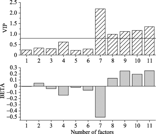
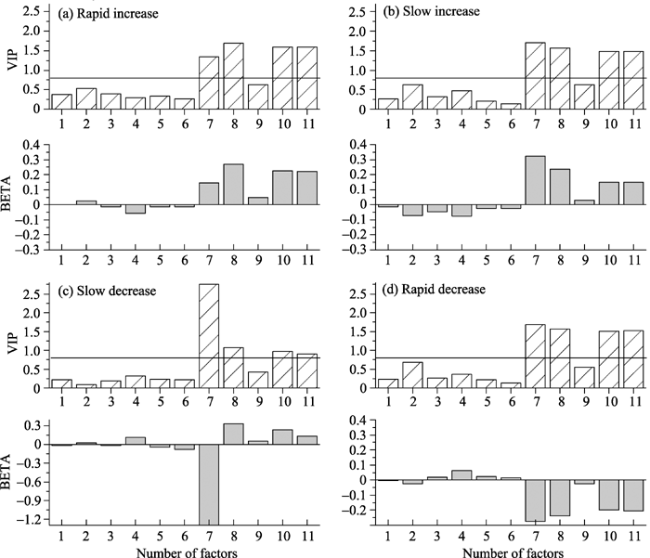
Studying the change in population distribution and density can provide important basis for regional development and planning. The spatial patterns and driving factors of the change in population density in China were not clear yet. Therefore, using the population census data in 2000 and 2010, this study firstly analyzed the change of population density in China and divided the change in all 2353 counties into 4 types, consisting of rapid increase, slow increase, slow decrease and rapid decrease. Subsequently, based on the partial least square (PLS) regression method, we recognized the significant factors (among 11 natural and social-economic factors) impacting population density change for the whole country and counties with different types of population change. The results showed that: (1) compared to the population density in 2000, in 2010, the population density in most of the counties (over 60%) increased by 21 persons per km2 on average, while the population density in other counties decreased by 13 persons per km2. Of all the 2353 counties, 860 and 589 counties respectively showed rapid and slow increase in population density, while 458 and 446 counties showed slow and rapid decrease in population density, respectively. (2) Among the 11 factors, social-economic factors impacted population density change more significantly than natural factors. The higher economic development level, better medical condition and stronger communication capability were the main pull factors of population increase. The dense population density was the main push factor of population decrease. These conclusions clarified the spatial pattern of population change and its influencing factors in China over the past 10 years and could provide helpful reference for the future population planning.

Cite this article

WANG Lu , FENG Zhiming , YANG Yanzhao . The change in population density from 2000 to 2010 and its influencing factors in China at the county scale[J]. Journal of Geographical Sciences, 2015 , 25(4) : 485 -496 . DOI: 10.1007/s11442-015-1181-z

1 Introduction

Population distribution, as a representative of the pattern of where people live, is an important research content in population geography (Zhu, 1980; Hu and Zhang, 1986; Li and Chen, 2009). Along with recent economic development, rapid urbanization, and the change in population policy, the pattern of population distribution in China has changed quickly over the past several decades (China Development Research Foundation, 2010; National Health and Family Planning Commission of China, 2011). Studying the change in patterns of population distribution and its influencing factors can not only help to clarify the process of population change, but also recognize the driving forces of regional population change.
The study about the change in population distribution occupies an important position in population geography. In general, regional population growth is not only affected by natural growth, but also by mechanical growth of population (Li and Chen, 2009). Many studies use demographic data such as age structure and fertility rate to analyze the natural population growth (Wang and Wei, 2003; Chen, 2006; Chen et al., 2006). With respect to mechanical growth of population, researchers use push-pull migration laws to study the causes of population growth (Wang and Wei, 2003; Cain et al., 2007; Xiao, 2010). For example, adverse living conditions such as overpopulation, unpleasant climate and dirty environment would push people to move out. On the contrary, favorable living conditions such as massive employment opportunity, pleasant climate and attractive lifestyle would pull people to move in (Bouvier et al., 1977). The population policies also impact population mobility (Lu, 1990; Cai, 1990; Feng and Zhou, 2003; Li and Chen, 2009). For instance, the regional differences in wage rate, medical and educational facilities have direct impacts on population migration (Zhu et al., 2002; Zhu and Zeng, 2004; Xiao, 2010); the industrial structure could affect regional population growth since labor absorption capacity varies among different industries (Zhu, 2002). Furthermore, internal traits of humans such as ages, genders, personality and level of education are also important influencing factors (Xiao, 2010).
From the methodological point of view, the frequently-used methods for studying the population growth consist of meta-analysis, questionnaire survey, theoretical analysis and statistical analysis. The meta-analysis method refers to the method that focuses on contrasting and combining results from different studies, in the hope of identifying the common factors impacting population change (Li, 2001; Wang and Ye, 2004). A weakness of this method is that sources of bias are not controlled by the method: a good meta-analysis of badly designed studies would still result in bad statistics. Questionnaire survey is a method to find out detailed information about lots of migrating peoples in small regions (Wu, 2013). Theoretical analysis method is usually to establish theoretical models such as push-pull laws to explain migration process. A potential pitfall of this method is that the established models might have difficulties in verifying (Xiao, 2010). Statistical analyses are the methods to analyze the relationship between regional population change and its influencing factors through correlation analysis, principal component analysis (PCA) or simple regression analysis etc. (Zhu, 2002; Zhu and Zeng, 2004; He and Wang, 2007; Li and Chen, 2009). Since there might be auto-correlation among independent variables, some studies used the model with lagged variables to address this problem (Beeson and DeJong, 2002; Zhu and Zeng, 2004; Rappaport, 2004), while others ignored the problem (Zhu et al., 2001; Zhu, 2002; Li and Chen, 2009).
To date, the studies about the population change and its influencing factors in China mainly focused on small regions (e.g. a specific city or province), while the studies on national scale were lacking. In addition, most of previous studies only analyzed the impacts of social-economic factors but ignored natural factors. In order to fill in these gaps, this study firstly analyzed the spatial pattern of change in population density on national and regional scales based on the China’s population census data in 2000 and 2010. Subsquently, we selected 11 factors both in natural and social-economic fields and used partial least squares regression (PLS) method to analyze the relationship between the change in population density and these factors. The objective of this study is to clarify the spatial patterns of population change in China and its main influencing factors.

2 Materials and methods

2.1 Data and preprocessing

The population data used in this study are permanent population data derived from population census of China in 2000 and 2010 at the county scale. For the natural and social-economic factors, the data sources are shown in Table 2. According to administrative division of China in 2010, totally 2353 counties were investigated. Because the administrative division of China in 2000 was different from that in 2010, we recalculated the data of each county in 2000. For the counties which have different boundaries in 2000 compared with 2010, we firstly converted the vector data in 2000 into raster data at 1 km spatial resolution. Then we summed up the raster value (2000) in grid cells of each county according to the administrative division in 2010.

2.2 Analysis of population change characteristics in China at the county scale

Through calculating the rate of change in population density (relative to national mean) for each county, we divided the change in 2353 counties into 4 types so as to reveal the regional difference in population change (Table 1). The equation for calculating the relative rate of change in population density is:
where Fj is relative rate of change in population density for county j; dj(2000) and dj(2010) are the population density for county j in 2000 and 2010, respectively; D2000 and D2010 are population density for the whole nation in 2000 and 2010, respectively. The classification rule for the change in population density is shown in Table 1.
Table 1 Classification rule for the change in population density at the county scale
Types for change in population density Abbreviation Classification rule
Rapid increase RI Fj>1
Slow increase SI 0≤Fj≤1
Slow decrease SD -1≤Fj<0
Rapid increase RD Fj<-1

2.3 Selection of factors influencing change in population density

The differences between population density in 2000 and 2010 for each county were chosen as response variables. Based on the previous studies (Zhu, 2002; Yue et al., 2005; Feng et al., 2008), 11 natural and social-economic factors which might affect the change of population density were chosen as predictor variables (Table 2). Among all the natural indicators, the relief degree of land surface (RDLS) (Feng, 2008) and the normalized difference vegetation index (NDVI) derived from satellite image can reflect regional terrain conditions and vegetation status, respectively. Mean annual temperature and precipitation can reflect regional climatic conditions and have direct impacts on comfort level of local residents (Bai et al., 2009). Total water resources and grain output can indicate amount of water resources and crop production capacity, respectively. Among social-economic factors, initial density of population in 2000 could reflect the basic condition of population distribution for each county; gross domestic product (GDP), length of transport routes, and the numbers of telephones and hospital beds can respectively show the level of regional economic development, traffic accessibility, capability of telecommunication and health security. All these indicators were selected as the potential factors impacting regional population growth.
Table 2 Potential factors influencing the change in population density and their data sources
Category No. Name Unit Description Data source
Natural factors 1 RDLS Mean RDLS for each county CGIAR-CSI
2 Total water
resources per km2
104 m3/km2 Total volume of surface water and groundwater divided by the area of each county Statistical yearbook
3 grain output per km2 t/km2 The total grain output for each country in 2000 divided by the area of each county Statistical yearbook
4 NDVI NDVI in 2000 at each county GIMMS
5 Average annual temperature °C Mean annual average temperature (1970~2000) at each county RESDC
6 Average annual precipitation mm Mean annual average precipitation (1970~2000) at each county RESDC
Social-
economic factors
7 Initial population density Persons/km2 Population density in 2000 at each county Statistical yearbook
8 Gross domestic product (GDP) density 104 yuan/km2 GDP divided by the area of each county in 2000 Statistical yearbook
9 Length of transport routes per km2 km/km2 Total length of railways in operation, highways and inland waterways in 2000 divided by the area of each county Statistical yearbook
10 Telephones density telephones/km2 The number of telephones in 2000 divided by the area of each county Statistical yearbook
11 Hospital beds density beds/km2 The number of beds in medical and health care institutions in 2000 Statistical yearbook

CGIAR-CSI(Consultative Group on International Agricultural Research website: http://srtm.csi.cgiar.org/ SELECTION/inputCoord.asp; RESDC (Data Center for Resources and Environmental Sciences of Chinese Academy of Sciences): http://www.resdc.cn/english/default.asp; Statistical yearbooks refer to National Bureau of Statistics of China, 2001a; National Bureau of Statistics of China, 2001b. Most of the factors are normalized by dividing the area of each county.

2.4 Partial least squares regression

Partial least squares (PLS) regression is an effective model to find the aspects of the signal in one response matrix (Y) that are directly related to signals in another matrix (X) of predictor variables (de Jong, 1993; Chong and Jun, 2005; Luedeling and Gassner, 2012). PLS regression could combine the advantages of Principal Component Analysis (PCA), Canonical Correlation Analysis (CCA) and Linear Regression Analysis (LRA). It works on the principle of variable compression and then gives the most important linear combinations of the original X. Moreover, PLS regression can avoid deviations caused by autocorrelation among predictor variables. Therefore, PLS regression could provide improved results and support richer and deeper data information than conventional analysis. The equations of PLS regression are:
where:
1) X is an n-by-p matrix of predictor variables, with rows corresponding to observations and columns to variables. X0 is standardized X calculated by subtracting off column means and dividing column standard deviations. is the PLS approximation to X0.
2) Y is an n-by-1 response matrix. Y0 is standardized Y calculated by subtracting off column means and dividing column standard deviation. is the PLS approximation to Y0.
3) XS is an n-by-ncomp orthonormal matrix with rows corresponding to observations and columns to components.
4) W is a p-by-ncomp matrix of PLS weights.
5) XL is a p-by-ncomp matrix of predictor loadings, where each row contains coefficients that define a linear combination of PLS components that approximate the original predictor variables.
6) YL is a 1-by-ncomp matrix of response loadings, where each row contains coefficients that define a linear combination of PLS components that approximate the original response variables.
PLS regression uses the least square method to estimate each parameter (including W, XL and YL). Meanwhile, PLS regression produces two major outputs: the variable-importance- in-the- projection (VIP) and the model coefficients (Beta). The equation of VIP is:
where VIPj is the VIP value for the j-th variable. PVk is the percentage of variance explained in Y by the k-th component. The variable with higher VIP value is more important for explaining variation in the dependent variable. Variables with a VIP value greater than 0.8 are commonly considered important and significant (Wold, 1995). The equation of Beta is:
where Beta is the PLS regression coefficients matrix (p×1). Res is the response residuals. The variable with a higher Beta value suggests that it has a stronger impact on response variable. The positive Beta indicates a promoted effect, which means that positive deviation in the independent variable is correlated to a high growth in the population. On the contrary, the negative Beta indicates a prohibitive effect, which means that positive deviation in the independent variable is correlated to a low growth or a negative growth in the population.
In this study, the response matrix is a column including differences in population density between 2000 and 2010 for each county. n equals to 2353, because China has 2353 counties. The predictor variables X is an 11-by-2353 matrix including the 11 factors mentioned above. The analysis was restricted to two components (ncomp=2) to ensure comparability of results across analyses and to avoid over fitting. All the analyses were implemented in the Matlab (Version 7.11.0.584) programming language.

3 Results and analysis

3.1 Spatial pattern of the change in population density from 2000 to 2010

Compared with the population density in 2000, the population density in 1449 counties had increased in 2010 (Figure 1). The area and population for all the counties with increased population density accounted for 66.7% and 68.2% of the whole nation’s area and population, respectively. Among 1449 counties with increased population density, 589 belonged to slow increase (SI) type (increased by 6.2 persons per km2 on the average); the other 860 belonged to rapid increase (RI) type (increased by 25.6 persons per km2 on the average). With regard to the spatial distribution, RI counties were mainly distributed in Beijing-Tianjin-Hebei economic zone, Yangtze River Delta, Pearl River Delta, arid region of Northwest China and Tibet Plateau.
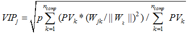
Figure 1 The spatial pattern of the change in population density in China from 2000 to 2010
From 2000 to 2010, the population density in 904 counties decreased (Figure 1). The area and population for all the counties with decreased population density accounted for 33.3% and 31.8% of the whole nation’s area and population, respectively. Among 904 counties with decreased population density, 458 belonged to slow decrease (SD) type (decreased by 4.9 persons per km2 on the average); 446 belonged to rapid decreased (RD) type (decreased by 24.0 per km2 on the average). These SD and RD counties were mainly distributed in populous provinces (e.g. Sichuan, Hubei, Anhui and Henan), municipality (e.g. Chongqing), old urban area of metropolis (e.g. Shanghai) and border areas in Northeast China (Figure 1).

3.2 Factors influencing change in population density at the national scale

PLS method was applied to calculate the importance of each factor in influencing the population density change for all counties in China. There were 5 factors whose VIP values were more than 0.8 and all of them were social-economic factors (Figure 2), including initial population density (VIP=2.19), hospital beds density (VIP=1.34), the telephones density (VIP=1.16), length of transport routes per km2 (VIP=1.11) and GDP density (VIP=0.98). Among these five factors, the BETA value of initial population density was negative (Figure 2), suggesting the larger initial population density would slow the speed of population growth. Other 4 factors showed positive impacts on the change in population density, which means that the higher values of these factors can promote population agglomeration. For the natural factors, the VIP values were all less than 0.8. Therefore, the impacts of natural factors on the change in population density were not significant at the national scale.
Figure 2 VIP and BETA values for the factors influencing population density change (2000-2010) at the national scale. Numbers of factors are shown in Table 2

3.3 Factors influencing change in population density at the regional scale

By employing PLS method to calculate the VIP and BETA values of each factor for counties belonging to 4 types, the factors influencing the change in population density for respective types of counties were analyzed (Figure 3).
For RI counties, the factors with VIP value more than 0.8 were all social-economic factors, including GDP density (VIP=1.69), telephones density (VIP=1.60), hospital beds density (VIP=1.60) and initial population density (VIP=1.34). All these factors had positive impacts on population growth (Figure 3a).
For SI counties, the factors with VIP value more than 0.8 were all social-economic factors, consisting of initial population density (VIP=1.70), GDP density (VIP=1.57), hospital beds density (VIP=1.48) and telephones density (VIP=1.47). Similar to RI counties, all significant influencing factors had positive impacts on population growth (Figure 3b).
For SD counties, 3 social-economic factors, including GDP density (VIP=1.08), telephones density (VIP=0.97) and hospital beds density (VIP=1.52) had significantly positive impacts on population growth. Besides, the VIP value of initial population density was more than 0.8 (VIP=1.68), but it had a negative impact on population growth. The VIP values of all natural factors were less than 0.8. Thus the impacts of natural factors on the change in population density are not significant for SD counties (Figure 3c).
For RD counties, the factors with VIP value more than 0.8 were all social-economic factors, including initial population density (VIP=1.68), GDP density (VIP=1.57), hospital beds density (VIP=1.53) and telephones density (VIP=1.51). All these factors had negative impacts on population growth (Figure 3d).
Figure 3 VIP and BETA values of factors influencing change in population density (2000-2010) for 4 types of counties. Numbers of factors are shown in Table 2

4 Discussion

In general, our results indicated that both natural and social-economic factors have certain impacts on the population growth. Furthermore, the strength of impacts of social-economic factors was much greater than the natural factors. Therefore, the population growth in China in recent decade can be mainly attributed to the social-economic factors.
(1) For counties with increased population density (including RI and SI counties), GDP density, telephones density and hospital beds density had significantly positive impacts on population growth, while the impacts of natural factors were not significant. Thus higher level of economic development, capacity of telecommunication and health security could pull people to move in. This result was consistent with the general understanding that people was inclined to migrate to affluent areas, because higher GDP corresponded with advanced economies, higher level income and better living conditions. Additionally, higher capacity of telecommunication could not only accelerate the economic information exchange within the region, but also provide information (e.g. the employment opportunity and commodity trading) for external labor markets. Furthermore, abundant health care facilities could provide both native and non-native population with good-quality medical care and improve the recovery rates and survival rates of some diseases. In addition, the results showed that initial population density had a significantly positive impact on population density growth for both SI and RI counties. This result was in contradiction to the result on national scale. The reason might be that the pulling forces caused by higher level economic development and capacity of telecommunication and health security were much greater than the pushing force caused by higher population density (Table 3).
Table 3 Average GDP, numbers of telephones and hospital beds for respective types of counties
Types of Change in
population density
Population density
(persons/km2)
GDP
(108 yuan)
Telephones number (104) Hospital beds
Number (104)
Rapid decrease 562.43 23.86 5195.63 941.83
Slow decrease 468.48 27.52 5921.12 1054.13
Slow increase 541.94 30.42 6731.72 1062.21
Rapid increase 608.54 62.35 11357.14 1801.03
(2) For SD counties, initial population density had a significantly negative impact on population growth while GDP density, telephones density and hospital beds density had positive impacts. These results suggested that for SD counties, the higher initial population density would push the local residents to move out and this pushing force was stronger than the pulling forces caused by higher regional economic development level and capacity of telecommunication and health security. Actually, the counties with dense population would make the local residents face more resource-environmental pressure or higher pressure of life, e.g. limited employment opportunities and higher strength of competition.
(3) For RD counties, initial population density, economic density, telephones density and hospital beds density all had negative impacts on population growth. Specially, the impacts of level of economic development, capacity of telecommunication and health security were different with our expectation. This is because the result was drawn from the PLS regression only using the data of RD counties while the migrations among different types of counties were ignored. As shown in Figure 1, most RD counties were located in populous provinces (such as Sichuan, Hubei, Anhui and Henan). In these populous provinces, the level of economic development was significantly lower than that in SI or RI counties (Table 3). Thus the pushing forces of higher level economic development, capacity of telecommunication and health security for RD counties resulted from the pulling forces of these factors for developed area (RI or SI counties). In fact, on national scale (all types of counties were included), higher level economic development, and capacity of telecommunication and health security had significantly positive impacts on population growth (Figure 2).
The spatial distribution of change in population density found in this study was consistent with the results from other studies. For example, a previous study showed that population density in Tibet Plateau had significantly increased in recent years due to high fertility rate (Fan and Wang, 2005). Except Tibet Plateau, the great change in population density was mainly caused by migration. Several studies found that populous provinces such as Sichuan, Henan and Hubei had the largest number of out-migrants, while Guangdong, Shanghai, Beijing and Zhejiang had most immigration (Cai, 2007; Zou, 2011). These results confirmed the spatial distribution of population change shown in this study (Figure 1). With respect to the reasons for population change, previous studies also indicated that for regions with decreased population, higher initial population density was the pushing forces for people to move out; for regions with increased population density, high level of economic development was the main pulling force (Wang and Wei, 2003; Zhu and Zeng, 2004).
In addition, this study did not discuss the effect of policy on population growth since it was difficult to quantify. In fact, policy might have certain impacts on regional population growth. For example, the great decreases of population in provinces such as Sichuan and Hubei were caused not only by migration, but also by relatively strict one-child policy (Guo et al., 2003). The decreases of population in old urban area of metropolises were directly related to policies of urban land use, housing and new zone development. The paid use of land in urban area and favorable revenue in development zones promoted lots of enterprises to move from urban central area to suburbs; the implementation of commercial housing systems urged citizens (especially middle class) to purchase affordable housing in the suburb (Liu and Zheng, 2004).

5 Conclusions

Using the population census data in 2000 and 2010, this study firstly analyzed the changing characteristics of population density in China. Also, we found out the important factors influencing the change in population density on national and regional scale by using PLS regression method. The main conclusions are as follows:
(1) With respect to the change in population density from 2000 to 2010, the proportions of RI, SI, SD and RD counties in all the 2353 counties were 36.5%, 25.0%, 19.5% and 19.0%, respectively. The counties with increased population density were distributed over the whole nation. Especially in Beijing-Tianjin-Hebei economic zone, Yangtze River Delta and Pearl River Delta, the population density increased most significantly. The counties with decreased population density were mainly distributed in populous provinces (e.g. Sichuan, Hubei, Anhui and Henan), municipality (e.g. Chongqing), old urban area of metropolis (e.g. Shanghai) and border areas in Northeast China.
(2) With respect to the factors influencing the change in population density, the social-economic factors played the predominant role in population growth, while the impacts of the natural factors were weak. Higher level of economic development and capacity of telecommunication and health security were the main factors pulling people to move in while higher initial population density was the main limiting factor for population growth and agglomeration.

The authors have declared that no competing interests exist.

1
Bai Q, Huo Z, He Net al., 2009. Analysis of human body comfort index of 20 tourist cities in China.Chinese Journal of Ecology, 28(8): 1607-1612. (in Chinese)

2
Beeson P E, Dejong D N, 2002. Divergence.Contributions in Macroeconomics, 2(1): 1.

3
Bouvier L F, Shryock H S, Henderson H W, 1977. International migration: Yesterday, today, and tomorrow.Population Bulletin, 32(4): 1-42.

4
Cai J, 1990. China’s population movement on province scale and its impacts on urbanization.Geographical Research, 9(2): 122-129. (in Chinese)

5
Cai J, Wang G, Yang Z, 2007. Future trends and spatial patterns of migration in China.Population Research, 5(31): 9-19. (in Chinese)

6
Chen G, Cao G, Liu Yet al., 2006. The future population of Beijing: A projection on the population, human capital and urbanization using PDE Model.Market & Demographic Analysis, 12(4): 29-41. (in Chinese)

7
Chen W, 2006. Future trends of population in China from 2005 to 2050.Population Research, 30(4): 93-95. (in Chinese)

8
China Development Research Foundation, 2010. China Development Report 2010. Beijing: People’s Publishing House. (in Chinese)

9
Chong I, Jun C, 2005. Performance of some variable selection methods when multicollinearity is present.Chemometrics and Intelligent Laboratory Systems, 78(1): 103-112.

10
De Jong S, 1993. SIMPLS: an alternative approach to partial least squares regression.Chemometrics and Intelligent Laboratory Systems, 18(3): 251-263.

11
Fan J, Wang H, 2005. Spatial analysis of population development and discussion of sustainable urbanization in Tibet.Scientia Geographica Sinica, 25(4): 385-392. (in Chinese)

12
Feng J, Zhou Y, 2003. The growth and distribution of population in Beijing metropolitan area (1982-2000).Acta Geographica Sinica, 58(6): 903-916. (in Chinese)

13
Feng Z, Tang Y, Yang Yet al., 2008. Relief degree of land surface and its influence on population distribution in China.Journal of Geographical Sciences, 18(2): 237-246.

14
Guo Z, Zhang E, Gu Bet al., 2003. Diversity of China’s fertility policy by policy fertility.Population Research, 27(5): 1-10. (in Chinese)

15
He S, Wang J, 2007. The analysis of economical pulling factors for migrants in Beijing, Shanghai and Guangzhou after reform and opening.Northwest Population Journal, 28(3): 8-11. (in Chinese)

16
Hu H, Zhang S, 1986. Population Geography of China. Shanghai: East China Normal University Press. (in Chinese)

17
Li G, Chen X, 2009. Empirical research on influencing factors on population growth of Beijing-Tianjin-Hebei Metropolitan Region.Geographical Research, 28(1): 191-202. (in Chinese)

18
Li L, 2001. Internal population migration in China since the economic reforms: A review.Geographical Research, 20(4): 453-462. (in Chinese)

19
Liu B, Zheng L, 2004. Characteristics and motive force mechanism of city sub-urbanization in China.Theory Journal, (10): 68-70. (in Chinese)

20
Lu Y, 1990. Population movement and the change of regional economy pattern.Geographical Research, 9(1): 41-46. (in Chinese)

21
Luedeling E, Gassner A, 2012. Partial least squares regression for analyzing walnut phenology in California.Agricultural and Forest Meteorology, 158: 43-52.

22
National Bureau of Statistics of China, 2001a. Counties’ Economic Statistical Yearbook of China 2001. Beijing: China Statistics Press, 1-573. (in Chinese)

23
National Bureau of Statistics of China, 2001b. Urban Statistical Yearbook of China 2001. Beijing: China Statistics Press, 1-589. (in Chinese)

24
National Health and Family Planning Commission of China, 2011. Floating Population Development Report in China 2011. Beijing: China Population Publishing House, 1-249. (in Chinese)

25
Rappaport J, 2004. Why are population flows so persistent?Journal of Urban Economics, 56(3): 554-580.

26
Wang D, Ye H, 2004. A review of migration research in China after 1990.Population Journal, (1): 40-46. (in Chinese)

27
Wang G, Wei X, 2003. Decrease in population in central areas of metropolis and aging: An example in Jing’an District, Shanghai.Population Research, 27(4): 78-85. (in Chinese)

28
Wold S, 1995. PLS for Multivariate Linear Modeling. In: van de Waterbeemd H (eds.) Chemometric Methods in Molecular Design. Weinheim: VCH Verlagsgesellschaft mbH, 195-218.

29
Wu Y, 2013. Current situation and influence of border area population outflow survey analysis based on three border counties in Heilongjiang Province. Changchun: Jilin University, 2013. (in Chinese)

30
Xiao Z, 2010. Hypothesis on potential energy conversion of population migration in theory: Re-interpretation of the push-pull migration laws.Population & Economics, (6): 77-83. (in Chinese)

31
Yue T, Wang Y, Liu Jet al., 2005. Surface modelling of human population distribution in China.Ecological Modelling, 181(4): 461-478.

32
Zhu C, Gu C, Ma Ret al., 2001. The influential factors and spatial distribution of floating population in China.Acta Geographica Sinica, 56(5): 549-560. (in Chinese)

33
Zhu C, Gu C, Zhang W, 2002. Quantitative analysis on influential factors of urban floating population in China.Population Journal, (2): 9-12. (in Chinese)

34
Zhu N, Zeng Z, 2004. The determinants of urban population growth in China.Chinese Journal of Population Science, (5): 9-18. (in Chinese)

35
Zhu Z, 1980. Discussion on reasonability of China’s population distribution.Population Research, 4(3): 11-17. (in Chinese)

36
Zou X, 2011. Analysis of population movement and distribution based on sixth census.Population & Economics, (6): 23-33. (in Chinese)

Outlines

/