Orginal Article

Spatio-temporal association analysis of county potential in the Pearl River Delta during 1990-2009

  • MEI Zhixiong ,
  • XU Songjun , * ,
  • OUYANG Jun
Expand
  • School of Geography, South China Normal University, Guangzhou 510631, China

*Corresponding author: Xu Songjun, PhD and Professor, specialized in environmental ecology.E-mail:

Author: Mei Zhixiong, PhD and Associate Professor, specialized in GIS and spatial statistics. E-mail:

Received date: 2014-05-09

  Accepted date: 2014-06-05

  Online published: 2015-03-15

Supported by

National Natural Science Foundation of China, No.41001078;No.41271060

Copyright

Journal of Geographical Sciences, All Rights Reserved

Abstract

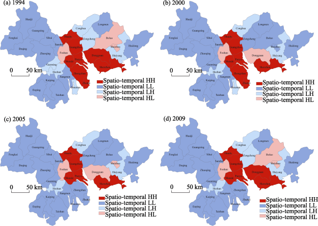
According to the highway data and some socioeconomic data of 1990, 1994, 2000, 2005 and 2009 of county units in the Pearl River Delta, this paper measured urban integrated power of different counties in different years by factor analysis, and estimated each county’s potential in each year by means of expanded potential model. Based on that, the spatio-temporal association patterns and evolution of county potential were analyzed using spatio-temporal autocorrelation methods, and the validity of spatio-temporal association patterns was verified by comparing with spatial association patterns and cross-correlation function. The main results are shown as follows: (1) The global spatio-temporal association of county potential showed a positive effect during the study period. But this positive effect was not strong, and it had been slowly strengthened during 1994-2005 and decayed during 2005-2009. The local spatio-temporal association characteristics of most counties’ potential kept relatively stable and focused on a positive autocorrelation, however, there were obvious transformations in some counties among four types of local spatio-temporal association (i.e., HH, LL, HL and LH). (2) The distribution difference and its change of local spatio-temporal association types of county potential were obvious. Spatio-temporal HH type units were located in the central zone and Shenzhen-Dongguan region of the eastern zone, but the central spatio-temporal HH area shrunk to the Guangzhou-Foshan core metropolitan region only after 2000; the spatio-temporal LL area in the western zone kept relatively stable with a surface-shaped continuous distribution pattern, new LL type units emerged in the south-central zone since 2005, the eastern LL area expanded during 1994-2000, but then gradually shrunk and scattered at the eastern edge in 2009; the spatio-temporal HL and LH areas varied significantly. (3) The local spatio-temporal association patterns of county potential among the three zones presented significant disparity, and obvious difference between the eastern and central zones tended to decrease, whereas that between the western zone and the central and eastern zones further expanded. (4) Spatio-temporal autocorrelation methods can efficiently mine the spatio-temporal association patterns of county potential, and can better reveal the complicated spatio-temporal interaction between counties than ESDA methods.

Cite this article

MEI Zhixiong , XU Songjun , OUYANG Jun . Spatio-temporal association analysis of county potential in the Pearl River Delta during 1990-2009[J]. Journal of Geographical Sciences, 2015 , 25(3) : 319 -336 . DOI: 10.1007/s11442-015-1171-1

1 Introduction

Massive spatio-temporal data (time and location specific data) are often available in real time with the extensive application of spatial information technologies. However, how to analyze these data and mine useful information concealed in them fully and effectively are crucial to the study of geographical spatio-temporal phenomena. The realistic objects or phenomena may not be distributed independently or randomly in space and time, but are often interacted with each other, and there is some spatio-temporal association between them for the formation of different spatial patterns (e.g. temporal association pattern, spatial association pattern and spatio-temporal association pattern). The spatio-temporal association is one of the primary reasons for the emergence, change and development of various spatial patterns (Cliff and Ord, 1981). Therefore, mining the spatio-temporal association relation concealed between objects or phenomena plays an important role in revealing the internal formation mechanism of different spatial patterns or differentiation.
At present, spatial analysis techniques have been widely used to mine the spatial patterns of objects or phenomena. They mainly include the application of some traditional spatial analysis methods such as quadrat analysis, kernel density function, nearest neighbor indicator and distribution function, etc. (Baddeley et al., 2000; Diggle et al., 2007; Sun et al., 2009; Yuan et al., 2010; Zheng et al., 2012) and Exploratory Spatial Data Analysis (ESDA) methods (Ma et al., 2004; Dallerba, 2005; Patacchini et al., 2007; Chen et al., 2008; Wan et al., 2011; Long et al., 2012; Cai et al., 2012). The traditional spatial analysis methods are only able to describe the overall spatial patterns of objects or phenomena, but cannot reflect local spatial heterogeneity. While the ESDA can reveal spatial dependence and spatial heterogeneity, but it depends completely on spatial sectional data and never involves temporal association effect, thus it is impossible to reflect the complicated spatio-temporal interaction between objects or phenomena. Moreover, the studies of spatial patterns based on the above methods mostly analyze the static spatial structure at single time-section, or compare the spatial structure at different time-sections to explore their whole evolution process. In nature, the spatial and temporal dimensions of the data remain separated in these studies, so it is required to establish a spatio-temporal association model which can effectively unify both of these in order to explore the spatio-temporal association patterns concealed in them. The actual geographical objects often present complicated temporal and spatial relationships, among which the spatio-temporal interaction is an essential factor (Wang, 2006), thus the spatio-temporal interaction should be taken into account when analyzing the association between geographical spatio-temporal data. Generally, the spatio-temporal data can be regarded as the time series dataset with spatial correlation, the spatio-temporal dependency and spatio-temporal heterogeneity are their two main characteristics (Cliff and Ord, 1975; Wang, 2006; Wang, 2008), and the spatio-temporal association patterns of geographical objects are formed under the combined effect of the spatio-temporal dependency and spatio-temporal heterogeneity (Cliff and Ord, 1981). Therefore, it is necessary to explore the spatio-temporal dependency and spatio-temporal heterogeneity in order to mine the spatio-temporal association patterns of geographical objects.
Developed on the basis of ESDA, the spatio-temporal autocorrelation techniques can explore spatio-temporal dependency and spatio-temporal heterogeneity, and thereby reveal the spatio-temporal interaction. As early as the 1970s, western scholars proposed the spatio-temporal autocorrelation concept (Cliff and Ord, 1975) and measurement method (Martin and Oeppen, 1975; Pfeifer et al., 1980) when modeling space-time series. Afterwards, the studies on spatio-temporal autocorrelation mainly concentrated in the following two aspects: (1) Considering the spatio-temporal correlation into spatio-temporal data models and their empirical analyses, such as the spatio-temporal series modeling and application in fields including real estate prices (Kelly et al., 1998; Pace et al., 1998, 2000; Tu et al., 2004; Sun et al., 2005; Smith et al., 2009; Asuncion et al., 2010; Brady, 2011), regional economy (Arbia et al., 2005; Robert et al., 2007), traffic (Kamarianakis et al., 2005; Han et al., 2007; Yue and Yeh, 2008), epidemic (Reynolds et al., 1988; Wang, 2006) and ecological environment (Cressie et al., 1997; Akito et al., 2011), etc. In these researches, the global spatio-temporal autocorrelation function is mainly employed to identify the space lag order and time lag period of the study objects, or 1-order spatial and temporal lags are directly set, then spatio-temporal regression or forecasting modeling is conducted. However, most of these researches do not consider the local spatio-temporal autocorrelation, and the spatio-temporal association structure characteristics of the study objects are not revealed. (2) Building some spatio-temporal autocorrelation statistical indices to study the spatio-temporal autocorrelation of the study objects (López et al., 2007; Hardisty et al., 2010; Cheng et al., 2012; Zhao et al., 2012; Chen et al., 2013). In researches of the second aspect, both global and local spatio-temporal autocorrelations are considered, and spatio-temporal dependency and spatio-temporal heterogeneity are all revealed. These studies have provided useful references for this paper, but the existing references indicate that the study of the spatio-temporal relationships between cities in a regional urban system under the perspective of spatio-temporal association is quite insufficient. Based on the above analysis and relevant former researches, this paper estimates county-level city potential indices of the Pearl River Delta using expanded potential model, and introduces the spatio-temporal autocorrelation methods considering both spatio-temporal effects to explore the spatio-temporal association structure and evolution of county potential from 1990 to 2009. Furthermore, this paper selects some typical units in which the spatio-temporal and spatial association patterns are obviously different to verify the accuracy of the spatio-temporal association analysis results by comparing with cross-correlation function (CCF). This paper would provide a new perspective for studying the relationships between cities in a regional urban system.

2 Study area and data

2.1 Study area

The Pearl River Delta (21º30′-23º40′N, 112º35′-113º57′E) in Guangdong Province, China, was chosen as the study area in this paper. It is in the southernmost part of the mainland in China, located in the south-central Guangdong Province and at the downstream Pearl River, as well as facing Hong Kong and Macao across the sea (Figure 1), belonging to the subtropical monsoon climate region. This region is one of China’s key economic central regions, and plays a significant strategic role in the national economic and social development. Since the reform and opening-up in 1978, especially after the 1990s, the economy and urbanization have undergone a rapid development and urban spatial agglomeration has enjoyed a sharp rise in the region (Chen et al., 2008). The land area of the Pearl River Delta is approximately 55,000 km2, accounting for 30.4% of Guangdong Province, and only 0.57% of China. In 2009, its GDP reached 82% of the province’s total and approximately 10% of national GDP, its resident population accounted for 49.7% of Guangdong Province and 4.09% of China, with a population density of 1019/km2, its urbanization level reached 80%, and its urban density grew to 10,140/million km2 (SBGD, 2010). The Pearl River Delta thereby became one of the Urban Agglomerations with high urban density and spatial elements agglomeration in China. For better comparative analysis, the range of the study area covers the entire administrative area of nine prefecture-level cities in the Pearl River Delta (Figure 1), including Longmen, Guangning, Deqing, Fengkai and Huaiji counties outsides the Pearl River Delta Economic Zone, and the basic area unit used in this paper is a county, a county-level city, or the urban district of a prefecture-level city (generally referred to as county units). Some units were merged according to the administrative division in 2009 and actual situations. Dongguan city and Zhongshan city, consisted of scattered townships, were taken as single units, respectively. Then a total of 30 area units were acquired (Figure 1).
Figure 1 The location of the study area and spatial distribution of county units

2.2 Data sources and processing

The studied basic indicator in this paper is the urban potential at county level calculated from the expanded potential model. It can reflect the agglomeration ability of a city in a related urban system (Xu et al., 2003), and such ability can promote all factors in the urban system to transfer and flow from the region with low agglomeration level to the region with high agglomeration level, so as to cause the spatial relationship of regional cities to undergo change. According to potential model, the data in this paper include two types, i.e. transportation network data and socio-economic data. The highway maps of the study area for 1990, 1994, 2000, 2005 and 2009 were collected from the Guangdong Province Map Publishing House, then the maps were processed via registration, digitization and topology to build a network dataset. By means of network analysis in GIS software, the shortest path distances among all units were acquired as the distance parameters in the potential model. This study therefore selected the five years corresponding to the road data as five time-sections, established the evaluation index system of urban integrated power at county level from four aspects including 24 indices listed in Table 1 based on the principles of completeness, comparability, hierarchy and data availability and referencing from the study by and Exploratory Spatial Data Analysis Chen et al. (2010). The original data in Table 1 were collected from the Guangdong Statistical Yearbook, China City Statistical Yearbook, China County (City) Economic and Social Statistical Yearbook of 1991-2010, and various statistical almanacs of related cities or spatial data. Individual missing data were obtained by interpolation calculation. After the original data were standardized by the Z-score, the urban integrated power indices of all county units were measured by factor analysis to be taken as the city size parameters in the potential model. According to the Technical Standard of Highway Engineering of the People’s Republic of China (JTGB01-2003) and actual situations, the speed limits for highways were set as 120 km/h on freeways, 80 km/h on national highways and 60 km/h on provincial and lower grade highways. The accessibility coefficient in the expanded potential model was calculated by the accessibility coefficient calculation formula. Based on the data acquisition, it is thus clear that the study period spans from 1990 to 2009.
Table 1 The evaluation index system of urban integrated power at county level
First-level indices Second-level indices
Urban scale level Urban non-agricultural population (x1) and urban built-up area (x2)
Urban economic level GDP (x3), GDP per capita (x4), gross industrial output value (x5), local government financial revenue (x6), local government financial expenditures (x7), savings deposits of urban and rural residents at the year-end (x8), total investment in fixed assets (x9), annual average wage of staff and workers (x10), total retail sales of consumer goods (x11), secondary industry output value (x12), tertiary industry output value (x13), proportion of tertiary industry output value in total output value (x14), foreign capital actually utilized (x15) and total foreign trade export value (x16)
Social development level Number of beds occupied per 10,000 persons in health institutions (x17), business volume of postal and telecommunication services (x18), business volume of postal and telecommunication services per capita (x19), number of persons with professional and technical titles (x20) and R&D expenditure (x21)
Infrastructure level Urban passenger traffic volume (x22), urban goods traffic volume (x23) and per capita length of highways in operation (x24)

3 Research methods

3.1 Expanded potential model

Due to individual unique nature of each city, even though two couples of cities are equal in the size and distance indices, their interaction may be different. According to the spatial interaction theory, the more complementarity, relativity and accessibility between two cities, the stronger interaction between the two cities. Considering data availability and quantifiability, the integrated economic correlation coefficient and accessibility coefficient among cities were introduced in this paper to expand the traditional potential model as follows, and the expanded potential model was used to estimate the potential index of each county:
where Ti is the potential value of city i, Tij is the interaction volume between cities i and j; dij is the distance between cities i and j, and the shortest highway distance between the two cities will be used in this paper; Pi and Pj are respectively the sizes of cities i and j, which will be expressed by the urban integrated power indices measured by factor analysis of the integrated power index system in Table 1, so as to avoid one-sidedness and excessive deviation problems caused by a single index; and b is the distance friction coefficient and can fall in the range 0.5 to 3, and its theoretical value should be 1 or 2 (Xu et al., 2003). Gu et al. (2008) found that the b value actually indicates the dimensional difference of spatial interaction, and b=2 is suitable to reveal the spatial interaction state in the provincial scale and regional urban system scale such as the Pearl River Delta Urban Agglomeration, and that b=1 is suitable for national scale. According to the practice, b=2 will be taken in this paper. In addition, dii denotes the distance between city i and itself, and can be expressed by the radius of a circle with equivalent area to city i (Xu et al., 2003); Rij represents the integrated economic correlation coefficient between cities i and j; and αi is the accessibility coefficient and can be calculated by the following formula:
where Ai is the accessibility value of city i and Ai=Di/Vi , Di and Vi are respectively the shortest highway distance and the average running speed between city i and another city.

3.2 Spatio-temporal autocorrelation methods

In the spatio-temporal autocorrelation analysis, spatio-temporal weight matrices are usually used to determine the spatio-temporal proximity between objects, and the spatio-temporal neighbors of each object are determined via its space-time lag terms. Cliff and Ord (1975) firstly proposed the spatio-temporal autocorrelation concept. Martin et al. (1975) obtained the spatio-temporal autocorrelation function and spatio-temporal partial autocorrelation function to measure quantitatively the spatio-temporal autocorrelation between objects (Pfeifer et al., 1980). Cliff and Ord (1981) also proposed a simple spatio-temporal autocorrelation index which requires setting a threshold constant in advance, but it is applied with difficulty due to its high subjectivity. Wang (2006) and López et al. (2007) expanded spatial Moran’s I to create more practical univariate spatio-temporal autocorrelation indices respectively. Hardisty et al. (2010) expanded the local spatial Moran’s I so as to obtain a local spatio-temporal autocorrelation statistic and developed a toolkit called LISTA-Viz, and applied it to an analysis of the 2009 H1N1 influenza in America, but the specific calculation formula was not given. Cheng et al. (2012) studied the spatio-temporal autocorrelation of road networks in London by means of spatio-temporal autocorrelation function and cross-correlation function (CCF). Zhao et al. (2012) expanded the CCF in order to establish a local spatio-temporal autocorrelation index with the same principle as that of CCF. Chen et al. (2013) improved the spatial Moran’s I so as to obtain a spatio-temporal Moran’s I index. The spatio-temporal autocorrelation statistics have two types of indices, i.e., global and local indices. Upon comparison, it is shown that the spatio-temporal Moran’s I indices including global and local statistical indices proposed by Wang (2006), López et al. (2007) and Chen et al. (2013), are basically consistent with each other in the form of function. Based on these references and actual situations, we first employ the spatio-temporal autocorrelation function and spatio-temporal partial autocorrelation function to determine the optimal time lag period and space lag order in the spatio-temporal autocorrelation process of county potential in the study area, then adopt the spatio-temporal Moran’s I indices (Wang, 2006; López et al., 2007; Chen et al., 2013) from the expansion of spatial Moran’s I to analyze the global spatio-temporal association characteristics and local spatio-temporal association structure of county potential. Furthermore, we verify the accuracy of the spatio-temporal association analysis results by comparing with the CCF.
3.2.1 Spatio-temporal autocorrelation function and spatio-temporal partial autocorrelation function
Supposing that Xt=[X1,X2,…XN]′ denotes the observation vector of N units at time t (t=1, 2, …, T), the spatio-temporal autocorrelation function of the sample data with h-order spatial lag and k-period temporal lag is (Martin et al., 1975; Pfeifer et al., 1980; Wang, 2008; Cheng et al., 2012):
where Zt and Zt-k respectively denote the standardized normal vectors of Xt and Xt-k, 
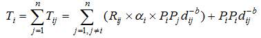
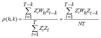
is the transposition of Zt, and Wh is the h-order spatial weight matrix.
In respect to the spatio-temporal partial autocorrelation function, the impacts of other spatio-temporal or intermediate variables are excluded, and the correlation between two spatio-temporal variables such as Xi+h,t and Xi,t-k can be accurately reflected. Its function form is defined as (Martin et al., 1975; Pfeifer et al., 1980; Wang, 2008):
where K and H are respectively the temporal and spatial lag orders, φkh is the spatio-temporal partial autocorrelation coefficient. This formula is a system of Yule-Walker equations including k equations, and its solving process refers to the study by Martin et al. (1975).
These two functions can only explore global spatio-temporal autocorrelation, and ignoring local spatio-temporal effect makes them helpless in revealing spatio-temporal heterogeneity, whereas they can be used to identify the time lag period and space lag order in the spatio-temporal autocorrelation process of the data. If the value decreases rapidly with the increases of the time lag period and space lag order, while the value displays as a truncation (close to 0) after the Kth period temporal lag and Hkth order spatial lag, then it is determined that the optimum time lag period is K and space lag order is Hk, in respect to the sample data (Martin et al., 1975; Pfeifer et al., 1980; Wang, 2008).
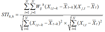
3.2.2 Spatio-temporal Moran’s I
The strength of correlation between an observation of unit i at time t-k and the same observations of units adjacent to unit i at time t can be effectively calculated by means of the univariate global spatio-temporal Moran’s I (denoted by STI) from the expanded Global Moran’s I. The calculation formula of the STI is as follows (Wang, 2006; López et al., 2007):
where Wij is an element of spatio-temporal weight matrix W, W can be replaced with spatial weight matrix directly for surface objects due to the temporal invariance of the adjacency relation of the polygon regions (Wang, 2006). Xi,t and Xj,t respectively denote the observations of units i and j at time t, Xi,t-k denotes the same observation of unit i at time t-k, and are the means of variable X at time t-k and variable X at time t, respectively. k and h respectively denote the time lag period and space lag order, and N is the number of sample units.
STIk,h is between -1 and 1, when STIk,h > 0, the global spatio-temporal autocorrelation of observations is positive and takes on spatio-temporal agglomeration with the adjacence of HH values or LL values in both time and space, and higher value of STIk,h presents stronger positive spatio-temporal autocorrelation. Otherwise, when STIk,h < 0, the global spatio-temporal autocorrelation is negative and presents a spatio-temporal scattered pattern of which the high and low values are adjacent, and the more STIk,h is close to -1, the stronger negative spatio-temporal autocorrelation it will appear. When STIk,h is equal or close to 0, it indicates that there is no spatio-temporal autocorrelation and observations take on spatio-temporal random distribution. The significance of STIk,h can be verified by the Z test.
The global index STIk,h is a synthesized measurement index for the overall spatio-temporal autocorrelation of all spatio-temporal objects and can disclose the spatio-temporal association pattern of the whole study area, but it neglects the potential instability of the spatio-temporal process and can not explore the difference between different spatio-temporal objects in the region (i.e., local spatio-temporal heterogeneity). For this purpose, the local index should be employed to reflect further the heterogeneous properties of this difference to reveal the local spatio-temporal association structure. The local spatio-temporal autocorrelation index STIi,k,h from the extension of local Moran’s I is adopted in this paper to explore the local spatio-temporal association structure of county potential in the study area, and its calculation formula is as follows (Wang, 2006; Chen et al., 2013):
where Zt,i is the normalized value of the observation of unit i at time t, Zt-k,j is the normalized value of the same observation of unit j adjacent to unit i at time t-k, and the meanings of other parameters are the same as those in Formula (5). The physical meaning of the local index STIi,k,h is similar to the global index STIk,h, but the value of STIi,k,h is not limited to between -1 and 1, determined according to the actual data.
Similar to the four types of local spatial association reflected by local Moran’s I, the local spatio-temporal association indicated by the STIi,k,h also has four different combinations which correspond to the four quadrants of the Moran scatterplot (Wang, 2006; Chen et al., 2013). In this paper, using the expression methods of local spatial association for reference, the four types of local spatio-temporal association are expressed as spatio-temporal HH, spatio-temporal LL, spatio-temporal HL and spatio-temporal LH: The spatio-temporal HH or LL means a local positive spatio-temporal autocorrelation exists between an object and its adjacent objects in both time and space, and there is a spatio-temporal conglomeration effect of the same high or low values. While the spatio-temporal HL or LH means local negative spatio-temporal autocorrelation, of which the high and low different values are adjacent, and the observations of spatio-temporal adjacent objects in the two types of local spatio-temporal association are of great disparity with each other, i.e., there is a local spatio-temporal heterogeneity in the observations.

4 Results and analysis

This study adopted the Z-score to standardize the data processing of original indices shown in Table 1, and used the factor analysis method to calculate the scores of the integrated power of each county in each year. To meet the requirement that the city size parameter in potential model is positive, this study referred to the study by Chen et al. (2010) and carried out data conversion of the original scores (possible negative) in the range 1 to 10 to obtain the scores of the integrated power, of which all values are positive and the original data size and order characteristics are not altered. Then the integrated economic correlation coefficients between counties were determined, the accessibility coefficients between counties in each year were measured by Formula (2), and the potential values of each county in each year were calculated using Formula (1) (Table 2).

4.1 Identification of the time lag period k and space lag order h

Because the county units in the study area are surface entities, it is suitable to use the contiguity rule including three methods of rook, bishop and queen to construct the spatial weight matrix. After comparison, the queen method was chosen to construct the spatial weight matrix of the study area. Then the spatio-temporal autocorrelation function and spatio-temporal partial autocorrelation function shown by Formulas (3) and (4) were used to identify the optimal time lag period and space lag order in the spatio-temporal autocorrelation process of county potential, so as to reveal accurately the time and space scales of the spatio-temporal association of county potential. The calculation results of the and of the sample data are respectively listed in Tables 3 and 4. As results shown in Tables 3 and 4, the value decreases rapidly with the increases of k and h, while the value is in the truncation state (close to 0) after space lag orders 0 and 1 and time lag period 1. It is thereby determined that the temporal lag period k=1 and spatial lag order h=1 are the most ideal time and space scales for analyzing the spatio-temporal association structure of the sample data.

4.2 Analysis of the global spatio-temporal association and evolution of county potential

Based on the above identified optimal time lag period and space lag order for the spatio-temporal association of the sample data, we calculated the global spatio-temporal auto correlation index STI1,1 of the sample data at forward first-order time lag and first-order space lag (i.e. k=1 and h=1) using Formula (5), and the results are shown in Table 5. The STI1,1 of the year 1990 was not calculated due to the lack of relevant data from the previous years.
Table 2 Values of urban potential at county level between 1990 and 2009
Study unit 1990 1994 2000 2005 2009 Study unit 1990 1994 2000 2005 2009
Guangzhou urban
district
0.4138 0.6424 0.6276 0.5735 0.5374 Jiangmen urban
district
0.0569 0.0647 0.0627 0.0578 0.0523
Huadu 0.1422 0.1143 0.1064 0.0899 0.1152 Taishan 0.0557 0.0447 0.0141 0.0268 0.0150
Conghua 0.0132 0.0161 0.0161 0.0147 0.0201 Kaiping 0.0613 0.0499 0.0207 0.0325 0.0204
Panyu 0.1605 0.1729 0.1393 0.1734 0.1103 Heshan 0.0467 0.0578 0.0514 0.0397 0.0420
Zengcheng 0.0312 0.0397 0.0302 0.0362 0.0475 Enping 0.0067 0.0084 0.0087 0.0069 0.0069
Shenzhen urban
district
0.1098 0.1323 0.2113 0.1667 0.1455 Foshan urban
district
0.1040 0.2631 0.2521 0.1753 0.1333
Zhuhai urban
district
0.0727 0.1317 0.0914 0.0701 0.0665 Shunde 0.1863 0.1660 0.1638 0.1491 0.1055
Doumen 0.0211 0.0251 0.0298 0.0191 0.0096 Sanshui 0.0420 0.0885 0.0707 0.0553 0.0538
Huizhou urban
district
0.0894 0.1677 0.0672 0.1080 0.1755 Gaoming 0.0161 0.0406 0.0373 0.0349 0.0344
Huidong 0.0285 0.0255 0.0141 0.0187 0.0184 Zhaoqing urban
district
0.0102 0.0140 0.0128 0.0146 0.0097
Huiyang 0.0239 0.0230 0.0216 0.0212 0.0181 Sihui 0.0163 0.0191 0.0166 0.0171 0.0178
Boluo 0.0393 0.1100 0.0154 0.0447 0.1044 Guangning 0.0064 0.0047 0.0032 0.0048 0.0048
Longmen 0.0043 0.0043 0.0030 0.0042 0.0046 Deqing 0.0053 0.0030 0.0039 0.0027 0.0041
Dongguan 0.0355 0.0891 0.1076 0.0929 0.1065 Fengkai 0.0044 0.0029 0.0032 0.0021 0.0035
Zhongshan 0.0660 0.0919 0.0785 0.0677 0.0663 Huaiji 0.0036 0.0029 0.0023 0.0031 0.0031
Table 3 Values of spatio-temporal autocorrelation function
k=1 k=2 k=3 k=4
h=0 0.9310 0.6492 0.3383 0.1025
h=1 0.2639 0.1504 0.0861 0.0204
h=2 0.0150 0.1076 0.0626 0.0062
Table 4 Values of spatio-temporal partial autocorrelation function
k=1 k=2 k=3 k=4
h=0 -0.6943 0.0623 0.0426 0.0032
h=1 -0.1420 0.0364 0.0025 -0.0011
h=2 -0.0717 0.0138 0.0157 -0.0019
As shown in Table 5, the global index STI1,1 in each year is significantly positive, which indicates that the global spatio-temporal association of county potential in the study area showed a positive effect during the study period, and presented spatio-temporal agglomeration, of which high observations tend to be adjacent to high observations in both time and space and so do the low observations as a whole. During 1994-2005, the STI1,1 value increased slowly, which implied that the positive spatio-temporal association was slowly strengthened and the overall disparity of county potential tended to decrease from 1994 to 2005. However, the STI1,1 value decreased in 2009, which showed the positive spatio-temporal association was decayed and the overall disparity of county potential expanded from 2005 to 2009, due to the fact that regional development during that period underwent a temporary fluctuation in the structural adjustment and integration stage.
Table 5 STI1,1 and its Z test of county potential at first-order time lag and space lag
Year 1994 2000 2005 2009
Global index STI1,1 0.2364 0.2388 0.2401 0.1897
Significant level 0.01 0.01 0.01 0.05
As a whole, the STI1,1 value of county potential in the Pearl River Delta in each year is not high, which indicates that the spatio-temporal association effect was not strong during the study period. The STI1,1 value did not vary much before 2005, but it varied much from 2005 to 2009, which implied that the overall spatio-temporal association pattern did not fluctuate significantly during 1994-2005, but it largely varied during 2005-2009.

4.3 Analysis of the local spatio-temporal association and evolution of county potential

The above global spatio-temporal association analysis based on the global index STI1,1 may hide the different spatio-temporal association situations in the region and can not locate the local spatio-temporal heterogeneity area, therefore the local index must be employed for further analysis. Using Formula (6), we calculated respectively the local spatio-temporal autocorrelation index STIi,1,1 for the potential of each county at forward first-order time lag and first-order space lag in 1994, 2000, 2005 and 2009 (except for 1990 due to the lack of relevant data from the previous years), and made the evolution figure of the local spatio-temporal association pattern by ArcGIS software (Figure 2). From the calculated results of the STIi,1,1 and Figure 2, we can see that most counties’ potential became involved in the local positive spatio-temporal autocorrelation in 1994, 2000, 2005 and 2009 with the percentage of 70%, 80%, 80% and 76.7% respectively, which indicated that the spatio-temporal association of county potential showed a positive effect on the whole and accorded with the global analysis results. In this study, the units which the spatio-temporal association properties did not change accounted for 73% of the total unit number. It showed that the local spatio-temporal association characteristics of most counties’ potential kept relatively stable, but the local spatio-temporal association in some counties changed.
As indicated in Figure 2:
(1) The distribution difference and its change of local spatio-temporal association types of county potential were obvious, the local spatio-temporal heterogeneity areas varied significantly. The spatio-temporal HH type units were located in the central zone and Shenzhen-Dongguan region of the eastern zone since 1994, but the spatio-temporal HH area (Zhongshan and Zhuhai urban district) in the south-central zone disappeared and that in the central zone shrunk to the Guangzhou-Foshan core metropolitan region only after 2000. The spatio-temporal LL type units mainly focused on the western and eastern zones during 1994-2000 and expanded to the western, eastern and south-central zones after 2000, among which the surface-shaped continuous distribution pattern of the LL type units in the relatively underdeveloped western zone kept relatively stable, and only one unit of Gaoming was added in 2000, the new LL type units (Doumen, Zhongshan and Zhuhai urban district) began to emerge in the south-central zone in 2005, the LL area in the eastern zone expanded during 1994-2000, but then gradually shrunk and scattered at the eastern edge in 2009, same as 1994. The distribution of the local spatio-temporal heterogeneity (spatio-temporal HL and LH) areas changed significantly, only Foshan urban district was always stable in the HL area, while the other HL type units varied frequently; the spatio-temporal LH type units were distributed around high potential counties with a ring-shaped distribution pattern, with the exceptions of Heshan, Conghua and Huiyang, which were always stable in the LH area, all other LH type units varied frequently.
Figure 2 Evolvement of local spatio-temporal association patterns of county potential
(2) There were obvious transformations in some counties among four types of local spatio-temporal association during the study period. As indicated in Figure 2: 1) There were 8, 7, 5 and 6 spatio-temporal HH type units in 1994, 2000, 2005 and 2009, respectively. Guangzhou urban district, Huadu, Panyu, Shunde and Shenzhen urban district were always of the HH type, Zhongshan and Zhuhai urban district were converted to the LL type since 2005, and Dongguan was of the HL type in 2000 and 2005, but returned to the HH type in 2009 (same as 1994). 2) There were 13, 17, 19 and 17 spatio-temporal LL type units in 1994, 2000, 2005 and 2009, respectively. Most counties in the western zone were always of the LL type. In the central zone, there was no distribution of this type but H-H spatio-temporal agglomeration was dominant during 1994-2000, nevertheless, changes occurred in 2005, namely Doumen was converted from the LH type to the LL type, Zhongshan and Zhuhai urban district were converted from the HH type to the LL type, and there was no change in the following years. The number of LL type units in the eastern zone was always changed, but Longmen and Huidong were always of the LL type. 3) There were 3, 2, 3 and 3 spatio-temporal HL type units in 1994, 2000, 2005 and 2009, respectively. Foshan urban district was always of the HL type. Huizhou urban district, except being of the LL type in 2000, was basically stable as the HL type. Boluo was of the HL type in 1994, the LL type in 2000 and 2005 and returned to the HL type in 2009. Dongguan was converted to the HL type since 2000 but exited from this type in 2009. 4) There were 6, 4, 3 and 4 spatio-temporal LH type units in 1994, 2000, 2005 and 2009, respectively. Conghua, Huiyang and Heshan were always of the LH type, and Gaoming was converted from the LH type to the LL type since 2000. Zengcheng was of the LH type in 1994, the LL type in 2000 and 2005 and returned to the LH type in 2009. Doumen exited from the LH type since 2005.
(3) The diversity of local spatio-temporal association among the three zones showed significant imbalance. The spatio-temporal HH type counties were dominant in the central zone during the study period, but after 2000 their number decreased slightly, their coverage narrowed, and the disparity between the south-central counties and central Guangzhou-Foshan core region expanded gradually; the local spatio-temporal association characteristics of the eastern counties varied significantly, the four local spatio-temporal association types converted frequently to each other, the disparity among the counties in the eastern zone first reduced and then expanded, but the agglomeration levels of some counties were improved; spatio-temporal LL type counties were dominant and relatively stable in the western zone, which showed that it was still difficult for them to rid themselves of low-level agglomeration. As a whole, the difference between the eastern and central zones tended to decrease, whereas that between the western zone and the central and eastern zones further expanded.

4.4 Comparison with spatial association structure and verification of the above analysis results

Based on the comparisons between Figures 2 and 3, the spatio-temporal and spatial association analysis results differ mainly in the following aspects:
(1) The changes of “HH” association areas are different in the two association analysis results. The HH type spatial association areas were concentrated in the central zone in the 1990s and later extended towards the eastern zone, e.g., Boluo of the eastern zone belonged to the HH spatial association area in 2009. However, the HH type spatio-temporal association areas were distributed in the central and eastern zones since 1994, the eastern HH spatio-temporal association area was centralized in Shenzhen and Dongguan but did not further extend towards the eastern zone, and Boluo had never been included in the spatio-temporal HH area.
(2) The changes of “HL” and “LH” association areas are different. Except for 1994, the local spatial heterogeneity areas did not change much. However, the distribution of local spatio-temporal heterogeneity areas changed significantly. Most spatio-temporal HL and LH units varied frequently except for Foshan urban district with a stable spatio-temporal HL type and three units of Heshan, Conghua and Huiyang were stable in the spatio-temporal LH area.
(3) Some units are different in terms of association type and transformation. As shown in Figure 3, Shenzhen urban district was always of the spatial HL type; Dongguan had been included in the spatial HH type since 1994; Boluo was of the spatial HL type in 1994, spatial LL type in 2000 and 2005, and converted to the spatial HH type in 2009; and Zhaoqing urban district was stable as the spatial LH type. However, in terms of spatio-temporal association analysis shown in Figure 2, Shenzhen urban district was always of the spatio-temporal HH type; Dongguan belonged to the spatio-temporal HH type in 1994, then converted to the spatio-temporal HL type but returned to the spatio-temporal HH type in 2009; Boluo was of the spatio-temporal HL type in 1994, spatio-temporal LL type in 2000 and 2005, but returned to the spatio-temporal HL type in 2009; and Zhaoqing urban district was stable as the spatio-temporal LL type. The two association patterns of these units are evidently different and typical.
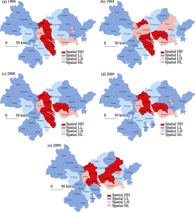
Figure 3 Evolvement of local spatial association patterns of county potential
Furthermore, the cross-correlation function (CCF) proposed by Box et al. (1976) was adopted to compare with the STI index of this paper to verify the validity of the spatio-temporal association analysis results. CCF, which can measure the cross correlation of samples in two regions at different time-sections, is a local measurement index for correlation between two series. Yue and Yeh (2008), Cheng et al. (2012) and Zhao et al. (2012) demonstrated through empirical examples that CCF can be used to determine the spatio-temporal autocorrelation of geographical objects at specified time lags. Given two series X and Y, the CCF at lag k is given as:
where is the cross-covariance between series X and Y at time lag k; and are the standard deviations of series X and Y, respectively; and are the means of series X and Y, respectively; and the CCF value is between -1 and 1 with 1 indicating perfect positive correlation, -1 perfect negative correlation and 0 no correlation. CCF can be used as a crosscorrelation function for multivariate statistical analysis, and used as an autocorrelation function for univariate analysis. The series X and Y in this paper represent the series constituted by a county’s potential and its spatial lag terms at two time-sections (the same observations at different time-sections) respectively, therefore is equivalent to auto-covariance.
Four typical units of Shenzhen urban district, Dongguan, Boluo and Zhaoqing urban district, in which the spatio-temporal and spatial association patterns are obviously different, were selected as examples to verify the validity of the above analysis results by comparing the STIi,1,1 with CCF. The optimal time lag period and space lag order for the spatio-temporal association of the sample data had been all identified as 1 in Section 4.1, so we calculated the CCF between the series constituted by each of these four units and its first-order spatial lag terms and the previous ones at time lag period 1 respectively, and conducted comparisons with the aforementioned local index STIi,1,1 (Figure 4).
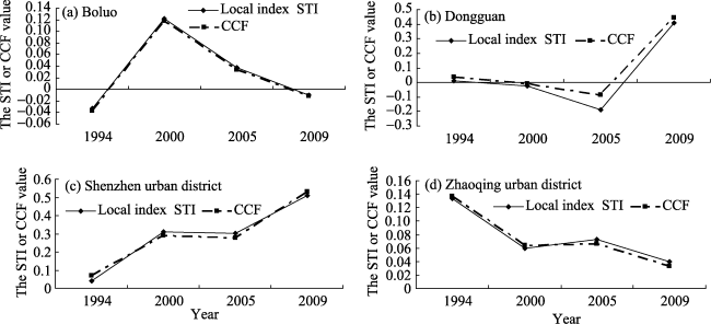
Figure 4 Comparison between STIi,1,1 index and cross-correlation function (CCF)
Figure 4 shows that the values of the CCF and STIi,1,1 of each unit were quite close to each other and their similarity was high in each year. The further correlation analysis between the two indices of Shenzhen urban district, Dongguan, Boluo and Zhaoqing urban district implied the following results respectively: CCF=0.967STIi,1,1+0.012 (R2 is 0.972), CCF= 0.918STIi,1,1+0.049 (R2 is 0.975), CCF= 1.009STIi,1,1-0.005 (R2 is 0.997) and CCF= 1.086STIi,1,1-0.008 (R2 is 0.977); the R2 of the two indices of these four units are all above 0.97, which indicates that the local spatio-temporal autocorrelation index STIi,k,h can capture the spatio-temporal autocorrelation of county potential in the study area accurately and effectively, and the two-way autocorrelation characteristics in both time and space existed in the county potential data during the study period. Therefore, the spatial association analysis only reflecting the static spatial autocorrelation at single time-section likely lost some valuable information in the exploration of the association patterns of county potential. However, the spatio-temporal association analysis considering both spatial and temporal autocorrelations can better reveal the dynamic autocorrelation structure in the sample data, and thereby is more comprehensive and more efficient than the spatial association analysis when mining the association patterns of county potential.

5 Conclusions and discussion

Conclusions from this research can be summarized as follows:
(1) The global spatio-temporal association of county potential in the Pearl River Delta showed a positive effect during the study period. But this positive effect was not strong, and it had been slowly strengthened from 1994 to 2005 and decayed from 2005 to 2009. The local spatio-temporal association characteristics of most counties’ potential kept relatively stable and focused on a positive spatio-temporal association especially the spatio-temporal LL association, however, there were obvious transformations in some counties among four types of local spatio-temporal association.
(2) The distribution difference of local spatio-temporal association types of county potential was obvious and had clearly changed. The spatio-temporal HH areas were located in the central zone and Shenzhen-Dongguan region of the eastern zone since 1994, but the coverage of the spatio-temporal HH area of the central zone shrunk to the Guangzhou-Foshan core metropolitan region only after 2000. The spatio-temporal LL areas were mainly distributed in the western and eastern zones during 1994-2000, and expanded to the western, eastern and south-central zones after 2000, among which the distribution of the spatio-temporal LL area in the western zone was relatively stable, a new spatio-temporal LL area emerged in the south-central zone since 2005, the spatio-temporal LL area in the eastern zone expanded during 1994-2000, but then gradually shrunk and scattered at the eastern edge in 2009. The distribution of the spatio-temporal HL and LH (spatio-temporal heterogeneity) areas changed significantly.
(3) Local spatio-temporal association analysis further indicated that there existed significant diversity among the three zones about the local spatio-temporal association characteristics. The spatio-temporal HH type counties were dominant in the central zone, but further centralized after 2000 and the disparity between the south-central counties and central core region expanded. The local spatio-temporal association characteristics of the eastern counties varied greatly and the agglomeration levels of some counties in the eastern zone were improved. The spatio-temporal LL type counties were always dominant in the western zone, which showed it was still difficult for them to rid themselves of low-level agglomeration. As a whole, the difference between the eastern and central zones tended to decrease, but that between the western zone and the central and eastern zones further expanded.
(4) According to the comparison with spatial association patterns and verification via CCF, spatio-temporal autocorrelation methods can efficiently mine the spatio-temporal association patterns of county potential, and can better reveal the complicated spatio-temporal interaction between counties in terms of potential than ESDA methods only considering spatial effect.
The spatio-temporal autocorrelation methods which attend to both spatial and temporal effects simultaneously were introduced in this paper to explore the spatio-temporal association patterns of county potential in the Pearl River Delta, and the spatio-temporal dependence and spatio-temporal heterogeneity and their change trends of county potential were accurately measured by the methods during 1990-2009. This research has resolved the problem that traditional spatial analysis methods and ESDA methods are only able to reflect the static spatial structure at single time-section but unable to reveal the complicated spatio-temporal interaction in the data, and effectively revealed the dynamic autocorrelation structure of county potential in the study area. The present study provides a new perspective for studying the relationships among regional cities and a decision-making reference for relevant policy makers. Nevertheless, being subject to data limitation, the data of consecutive years during the study period are not available, and the in-depth analysis of the influence degree of temporal fluctuation and spatial distribution on the change of the spatio-temporal autocorrelation indices has not yet been conducted. These aspects need to be further investigated.

The authors have declared that no competing interests exist.

1
Akito N, Takahisa Y, Asao Aet al., 2011. Spatiotemporal autoregressive models of country-level emission of transboundary pollutants. SSRN Working Paper Series, 1-36.

2
Arbia G,Basile R, Piras G, 2005. Using spatial panel data in modeling regional growth and convergence. ISAE Working Paper No.55: 1-31.

3
Asuncion B, Pilar G, Manuel S, 2010. Analysis of housing price by means of STAR models with neighbourhood effects: A Bayesian approach.Journal of Geographical Systems, 12(2): 227-240.

4
Baddeley A, Meller J, Waagepetersen R, 2000. Non- and semi-parametric estimation of interaction in inhomogeneous point patterns.Statistica Neerlandica, 54(3): 329-350.

5
Box G, Jenkins G, 1976. Time Series Analysis: Forecasting and Control. San Francisco: Wiley, 256-268.

6
Brady R, 2011. Measuring the diffusion of housing prices across space and over time.Journal of Applied Econometrics, 26(2): 213-231.

7
Cai Fangfang, Pu Lijie, Zhang Jianet al., 2012. Identification of spatial economic structure in Jiangsu province by applying exploratory spatial data analysis.Economic Geography, 32(3): 22-28. (in Chinese)

8
Chen Gangqiang, Li Xun, Xu Xueqiang, 2008. Spatial agglomeration and evolution of urban population in China.Acta Geographica Sinica, 63(10): 1045-1054. (in Chinese)

9
Chen Qunyuan, Song Yuxiang, 2010. Methods of dividing the boundary of urban agglomerations: Chang-Zhu-Tan Urban Agglomeration as a case.Scientia Geographica Sinica, 30(5): 660-666. (in Chinese)

10
Chen Shaokuan, Wei Wei, Mao Baohuaet al., 2013. Analysis on urban traffic status based on improved spatio-temporal Moran's I.Acta Physica Sinica, 62(14): 527-533. (in Chinese)

11
Cheng T, Haworth J, Wang J Q, 2012. Spatio-temporal autocorrelation of road network data.Journal of Geographical Systems, 4: 389-413.

12
Cliff A D, Ord J K, 1975. Space-time modelling with an application to regional forecasting.Transactions of the Institute of British Geographers, 64:119-128.

13
Cliff A D, Ord J K, 1981. Spatial Processes: Models and Applications. London: Pion.

14
Cressie N, Majure J J, 1997. Spatio-temporal statistical modeling of livestock waste in streams.Journal of Agricultural, Biological and Environmental Statistics, 2(5): 20-28.

15
Dallerba S, 2005. Distribution of regional income and regional funds in Europe 1989-1999: An exploratory spatial data analysis.Annals of Regional Science, 39(1): 121-148.

16
Diggle P J, Gómez-Rubio V, Brown P Eet al., 2007. Second-order analysis of inhomogeneous spatial point processes using case control data.Biometrics, 63(2): 550-557.

17
Gu Chaolin, Pang Haifeng, 2008. Study on spatial relation of Chinese urban system: Gravity model approach.Geographical Research, 27(1): 1-12. (in Chinese)

18
Han Weiguo, Wang Jinfeng, Gao Yigeet al., 2007. Forecasting and analysis of regional traffic flow in space and time.Journal of Highway and Transportation Research and Development, 24(6): 92-96. (in Chinese)

19
Hardisty F, Klippel A, 2010. Analysing spatio-temporal autocorrelation with LISTA-Viz.International Journal of Geographical Information Science, 24(10): 1515-1526.

20
Kamarianakis Y, Prastacos P, 2005. Space-time modeling of traffic flow.Computers & Geosciences, 31: 119-133.

21
Kelly R P, Barry R, Clapp Jet al., 1998. Spatio-temporal autoregressive models of neighborhood effects.Journal of Real Estate Economics, 17(1): 15-33.

22
Long Kaisheng, Zhao Yali, Zhang Honghuiet al., 2012. Spatial difference and its influencing factors in ecological land rent in China.Acta Geographica Sinica, 67(8): 1125-1136. (in Chinese)

23
López H F A, Chasco Y C, 2007. Time-trend in spatial dependence: Specification strategy in the first-order spatial autoregressive model.Estudios de EconomÍa Aplicada, 25(2): 631-650.

24
Ma Xiaodong, Ma Ronghua, Xu Jiangang, 2004. Spatial structure of cities and towns with ESDA-GIS framework.Acta Geographica Sinica, 59(6):1048-1057. (in Chinese)

25
Martin R L, Oeppen J E, 1975. The identification of regional forecasting models using space-time correlation functions.Transactions of the Institute of British Geographers, 66: 95-118.

26
Pace R K, Barry R, Clapp J Met al., 1998. Spatiotemporal autoregressive models of neighborhood effects.Journal of Real Estate Finance and Economics, 17(1):15-33.

27
Pace R K, Barry R, Gilley O Wet al., 2000. A method for spatial-temporal forecasting with an application to real estate prices.International Journal of Forecasting, (16): 229-246.

28
Patacchini E, Rice P, 2007. Geography and economic performance: Exploratory spatial data analysis for Great Britain.Regional Studies, 41(4): 489-508.

29
Pfeifer P E, Deutsch S J, 1980. A three-stage iterative procedure for space-time modeling.Technometrics, 22(1): 35-47.

30
Reynolds K M, Madden L V, 1988. Analysis of epidemics using spatio-temporal autocorrelation.Phytopathology, 78(2): 240-246.

31
Smith T E, Wu P, 2009. A spatio-temporal model of housing prices based on individual sales transactions over time.Journal of Geographical Systems, 11(4): 333-355.

32
Statistical Bureau of Guangdong Province( SBGD), 2010. Guangdong Statistical Yearbook 2010. Beijing: China Statistics Press. (in Chinese)

33
Sun H, Tu Y, Yu S M, 2005. A spatio-temporal autoregressive model for multi-unit residential market analysis.The Journal of Real Estate Finance and Economics, 31(2): 155-187.

34
Sun Tieshan, Li Guoping, Lu Minghua, 2009. Concentration and decentralization of population in the Beijing-Tianjin-Hebei metropolitan region and its determinants: A regional density function approach.Acta Geographica Sinica, 64(8): 956-966. (in Chinese)

35
Tu T, Yu S M, Sun H, 2004. Transaction-based office price indexes: A spatial-temporal modeling approach.Real Estate Economics, 32(2): 297-328.

36
Wan Luhe, Wang Shaowei, Chen Xiaohong, 2011. GeoDA-based spatial correlation analysis of GDP in Hadaqi industrial corridor.Geographical Research, 30(6): 977-984. (in Chinese)

37
Wang Jiaqiu, 2008. Space-time series data analysis and modeling [D]. Guangzhou: Sun Yat-Sen University. (in Chinese)

38
Wang Jinfenget al., 2006. Spatial Analysis. Beijing: Science Press, 76-78. (in Chinese)

39
Xu Xueqiang, Zhou Yixing, Ning Yuemin, 2003. Urban Geography. Beijing: Higher Education Press. (in Chinese)

40
Yuan Feng, Wei Yehua, Chen Wenet al., 2010. Spatial agglomeration and new firm formation in the information and communication technology industry in Suzhou.Acta Geographica Sinica, 65(2): 153-163. (in Chinese)

41
Yue Y, Yeh A G O, 2008. Spatio-temporal traffic-flow dependency and short-term traffic forecasting.Environment and Planning B, 35(5): 762-771.

42
Zhao Ling, Wang Jiaqiu, Deng Minet al., 2012. Spatial-temporal autocorrelation model of road network based on travelling time. Journal of Central South University (Science and Technology), 43(10): 4114-4122. (in Chinese)

43
Zhen Feng, Yu Yang, Wang Xiaet al., 2012. The spatial agglomeration characteristics of automotive service industry: A case study of Nanjing.Scientia Geographica Sinica, 32(10): 1200-1208. (in Chinese)

Outlines

/