Orginal Article

Two universal runoff yield models: SCS vs. LCM

  • LI Jun ,
  • LIU Changming , * ,
  • WANG Zhonggen ,
  • LIANG Kang
Expand
  • Key Laboratory of Water Cycle & Related Land Surface Processes, Institute of Geographic Sciences and Natural Resources Research, CAS, Beijing 100101, China

*Corresponding author: Liu Changming, Professor, specialized in hydrology and water resources. E-mail:

Author: Li Jun (1968-), PhD Candidate, specialized in hydrology and water resources. E-mail:

Received date: 2014-05-05

  Accepted date: 2014-06-10

  Online published: 2015-03-15

Supported by

National Natural Science Foundation of China, No.41271048

The Key Program of National Natural Science Foundation of China, No.41330529

Copyright

Journal of Geographical Sciences, All Rights Reserved

Abstract

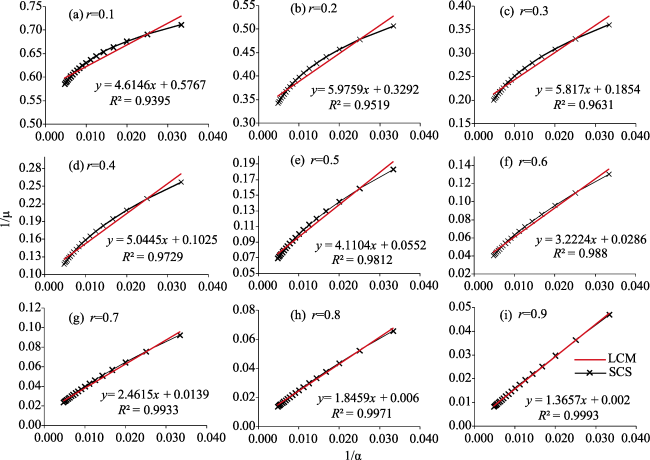
Runoff calculation is one of the key components in the hydrological modeling. For a certain spatial scale, runoff is a very complex nonlinear process. Currently, the runoff yield model in different hydrological models is not unique. The Chinese LCM model and the American SCS model describe runoff at the macroscopic scale, taking into account the relationship between total actual retention and total rainfall and having a certain similarity. In this study, by comparing the two runoff yield models using theoretical analyses and numerical simulations, we have found that: (1) the SCS model is a simple linear representation of the LCM model, and the LCM model reflects more significantly the nonlinearity of catchment runoff. (2) There are strict mathematical relationships between parameters (R, r) of the LCM model and between parameters (S) of the SCS model, respectively. Parameters (R, r) of the LCM can be determined using the research results of the SCS model parameters. (3) LCM model parameters (R, r) can be easily obtained by field experiments, while SCS parameters (S) are difficult to measure. Therefore, parameters (R, r) of the LCM model also can provide the foundation for the SCS model. (4) The SCS model has a linear relationship between the reciprocal of total actual retention and the reciprocal of total rainfall during runoff period. The one-order terms of a Taylor series expansion of the LCM model describe the same relationship, which is worth further study.

Cite this article

LI Jun , LIU Changming , WANG Zhonggen , LIANG Kang . Two universal runoff yield models: SCS vs. LCM[J]. Journal of Geographical Sciences, 2015 , 25(3) : 311 -318 . DOI: 10.1007/s11442-015-1170-2

1 Introduction

Calculation of runoff is one of the key processes in the hydrological simulation. Climate factors (i.e. rainfall intensity, duration, distribution) and land surface factors (i.e. soil types, vegetation, slope, etc.) have an important effect on runoff, and the formulas for runoff calculation are not unique in different hydrological models. Runoff could be investigated from both macroscopic and microscopic aspects. From microscopic point of view, the Richards equation with rigorous physical significance is usually used to calculate infiltration and runoff. From macroscopic point of view, there are three types of runoff: infiltration excess (Horton) runoff, saturated excess (Dunne) runoff, and mixed runoff. Runoff mechanisms have been well recognized, while how to calculate it remains controversial. For a certain spatial scale, the generation of runoff is a complex process. Due to different generation time for different water sources, the rapidly direct runoff forms as the preferential flow in large porous media always preferentially contributing to the peak flow. As long as the rainfall intensity exceeds the infiltration intensity, infiltration excess runoff will occur, no matter the soil is saturated or not. Therefore, it is necessary to consider the effect of infiltration excess runoff on the generation of peak flow. However, the infiltration in an area is not the same as that at a single point, and the infiltration excess runoff concentration is always accompanied by infiltration in the process of concentration along the surface. This phenomenon is called dynamic infiltration. For the dynamic infiltration, we carried out a series of artificial rainfall experiments in the field. The results showed that before overland flow occurs, when the rainfall intensity exceeds infiltration intensity, ponding first appears in the low-lying areas to gradually form the ponding layer, and with the increase of water pressure, runoff discharge increases, when the land surface is all covered by the excess runoff (i.e. overland flow appears in the whole area), the infiltration intensity becomes stable, and then the infiltration process steps into the stage of steady seepage. During the period of 1958-1978, in order to calculate and forecast the flood peak discharge in ungauged watersheds, Liu et al. performed the systematic study. Using portable devices for artificial rainfall, Liu et al. carried out a series of artificial rainfall experiments in the fields, with different land surface and soil wetness conditions in many places in China. According to the conservation law of energy, based on the analyses of the gravity, resistance and capillary force in the infiltration process, Liu et al. established an empirical equation to calculate the infiltration using rainfall intensity, land use/cover and soil moisture, and developed the LCM model that is suitable to the dynamic infiltration and runoff in China. Afterwards, based on the LCM model, coupled with other hydrological processes, we have independently developed a distributed hydrological model, named HydroInformatic Modeling System (HIMS) (Liu et al., 2005, 2008, 2009; Wang et al., 2004, 2005; Liang et al., 2012). HIMS has been widely tested for catchments under different natural conditions in both northern and southern China, Australia, and some parts of the United States. The modeling results were satisfactory. LCM parameters are very easy to measure using portable devices producing artificial rainfall, and the LCM model is also simple to be integrated into the distributed hydrological model, which has been the core module for runoff calculation in HIMS.
The Soil Conservation Service Curve Number (SCS model) method was developed by the United States Department of Agriculture (USDA) in 1954 for predicting direct runoff or infiltration from rainfall excess and is now known as the USDA Natural Resources Conservation Service (NRCS) (USDA, 1986). The transformation and generalization of the empirical relation of Mockus (1949) and the soil-vegetation-land-use (SVL) complex of Andrews (1954) yielded the SCS-CN method (Rallison and Miller, 1982) described in the Soil Conservation Service National Engineering Handbook Section 4 (SCS, 1956, 1964, 1971, 1985). The SCS model was developed from an empirical analysis of runoff at small catchments and hill slope plots monitored by the USDA. The SCS method has been widely used for estimating the approximate amount of direct runoff from a rainfall event in a particular area. In the 1990s, SWAT (Soil and Water Assessment Tool) also developed by USDA was used widespread, becoming a world famous model. The use of the SCS model in SWAT has made the SCS-CN method popular to calculate runoff (Reyes et al., 2007).
Apparently, the Chinese LCM model and the American SCS model were developed during similar period. Both models describe watershed runoff at the macroscopic scale, taking into account the relationship between total actual retention and total rainfall and having a certain similarity. However, there are few studies to analyze and compare these two models. In this study, we make a comparison between two runoff yield models using theoretical analyses and numerical simulations, in order to reveal their inherent relationship, and to discuss the macro-runoff mechanism in depth for the development of hydrological models.

2 Theory of models

2.1 SCS model

The SCS runoff curve number method represents the combined hydrologic effect of soil, land use, agricultural land management practices, hydrologic and antecedent soil moisture conditions (McCuen, 1982). The original SCS-CN method was documented in Section 4 of the National Engineering Handbook in 1956. This document was revised subsequently in 1964, 1965, 1971, 1972, 1985, 1993 (Mishra and Singh, 2003) and 2004 (SCS, 2004). This method is based on water balance equation and the two hypotheses to compute surface runoff in small agricultural watersheds (Mishra and Singh, 1999, 2002a, 2002b, 2003, 2004a, 2004b).
The SCS assumes a rainfall-runoff relation as:
where P is the total rainfall (mm), Ia the initial abstraction (mm), F the actual infiltration (mm), Q the direct runoff (mm), and S is the potential maximum retention or infiltration after runoff occurs (mm).
The actual retention, when the initial abstraction is considered, is:
Substituting equation (1) into (2) for Q yields:
The SCS assumes that Ia is a function of the maximum potential retention (S):
Ia is highly variable, correlated with soil and cover parameters (Patil et al., 2008). In many studies for small agricultural watersheds, an empirical Ia = 0.2S was used (SCS, 1985).
Substituting equation (4) into equation (3) gives:
where S can be estimated as:
in which CN is the runoff curve number (0 ≤ CN ≤100), which is a function of land use, antecedent soil moisture and other factors that affect runoff and retention. Figure 1 solves equation (5) for a range of CN and rainfall.
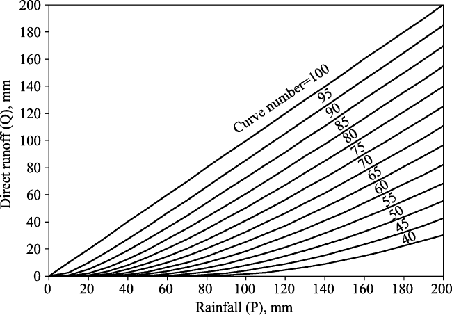
Figure 1 Solution of runoff equation (Cronshey, 1986)

2.2 LCM model

According to the analysis of storm runoff in small watersheds (Chen, 1966) and the artificial rainfall tests in the field (Liu, 1965), the losses of rainfall are mostly related to rainfall intensity α or rainfall duration t, and soil flow properties. Rate of losses μ was plotted against the rainfall intensity a (this relationship is similar to the rainfall versus losses curves obtained by Hicks (1944)), and the μ-a relationship (Liu and Wang, 1980) is quantified as:
where μ is the average intensity of the losses of rainfall on the ground in small watersheds, R is the coefficient of losses related to the kind of soil or soil flow properties, r is the index of the losses. We have called equation (7) the LCM model in HIMS (Liu et al., 2005, 2008, 2009).
It is noticeable that both R and r show the characteristics of terrain conditions, including vegetation and antecedent soil wetness. The values of R and r approach zero for impervious land surface (such as the surface of concrete), thus μ = 0, but for intensive pervious land surface both R and r approach 1. We analyzed the observations of our small experimental watersheds and the results of artificial experiments in the field. The values R and r are shown in Table 1.
Table 1 Values of parameters R and r for LCM model
Antecedent soil moisture Classification of the losses
II III IV V VI
Wet R 0.83 0.95 0.98 1.10 1.22
r 0.56 0.63 0.66 0.76 0.87
General R 0.93 1.02 1.10 1.18 1.25
r 0.63 0.69 0.76 0.83 0.90
Dry R 1.00 1.08 1.16 1.22 1.27
r 0.68 0.75 0.81 0.87 0.92

Note: Description of the terrain condition, i.e. II: clay, saline clay, thin layer of soil, and poor vegetation; III: sand clay and poor silt loam and poor vegetation, Gobi, vegetation, earth and rock hill regions with thin layer of soil; IV: silt loam and poor vegetation, earth and rock hill regions with thick layer of soil, the hill regions with thicket, grass land; V: silt and well vegetated forest; VI: sand, original forest with thick forest floor.

3 Comparison between the LCM model and the SCS model

3.1 Comparison of theory

For the SCS model, Q is given by substituting equation (1) into (2) to eliminate the parameter F, while the LCM model is used to calculate this F. Therefore, we can get F by eliminating Q from equations (1) and (2):
Apparently, equation (8) is still the SCS model, just in an alternative form.
For the LCM model, μ and α can also be calculated as:
In order to compare SCS and LCM, we set t = unit time (1 h) in LCM, then obtain:
Equation (10) shows that the SCS mode is a linear relationship between reciprocal of F and reciprocal of α, while equation (11) shows a nonlinear relationship between reciprocal of F and reciprocal of α for the LCM mode. By taking the one-order terms of a Taylor series expansion of equation (11) on the point, α=1/α0, we get:
To set α= [30, 210] mm / h, r = within [0.1, 0.9], we can attain optimal value of α0 for different r by numerical analysis of equation (12):
To set equation (12) = equation (10) item by item, we gain:
Based on the above derivation, we can obtain the relationship between parameters (R, r) of LCM and parameters (S) of SCS:
Equation (16) shows that the parameter R has a clear correlation with the parameter r in LCM.

3.2 Comparison of numerical simulations

Taking (1/α) as a global variable, rainfall α= [30, 210] mm / h, step length=10, r = [0.1, 0.9], step= 0.1, we plot out equation (11) (the LCM model) and fit the curve using a straight line which represents the SCS model. The results are shown in Figure 2.
Figure 2 Linear regression analysis of the LCM model (t=1 h; a = [30, 210] mm/h; 1/μ vs. 1/α)
Moreover, we analyze for shorter steps, taking rainfall α= [30, 210] mm / h, step length=1; r = [0.05, 0.95], step= 0.001, and the results are shown in Figure 3.
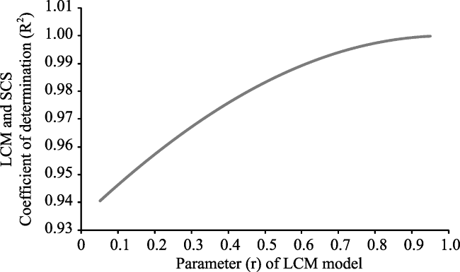
Figure 3 Coefficient of determination of the LCM and SCS models for different values of r (α= [30, 210] mm/h, step = 1; r = [0.05, 0.95], step= 0.001)
The comparison of theory (equation 14) and the comparison of numerical simulation (Figures 2 and 3) show that the SCS model is a simple linear representation of the LCM model. For r = [0.05, 0.95], the correlation coefficient (R2) is greater than 0.94, and the larger r is, the better fit we get.

3.3 Relationship of parameters between SCS model and LCM model

Figure 4 shows that R is not a single-valued function of CN. At the point (R, CN) = (6.36, 92), the curve appears twisted. However, when CN≤92, R becomes larger with the increase of CN. R and CN have uniqueness of correspondence with CN.
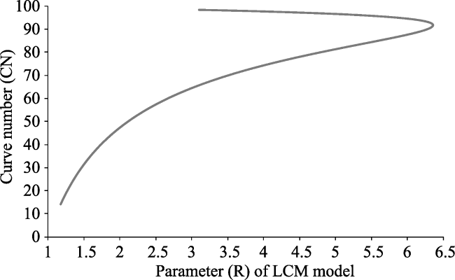
Figure 4 Relationship of R (LCM model) to CN (SCS model) (α=[30, 210] mm/h, step=1; r=[0.05, 0.95], step= 0.001)
Figure 5 shows that r is a single-valued function of the CN, the larger r, CN smaller. The r has α correspondence relationship with CN.
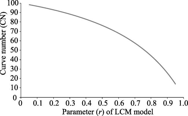
Figure 5 Relationship of r (LCM model) to CN (SCS model) (α= [30, 210] mm/h, step=1; r=[0.05, 0.95], step= 0.001).
Figure 5 shows a complex relationship between R and r. When r <0.23, R goes up with the increase of r. When r>0.23, R decreases with increasing r. When r>0.3, there is α linear relationship between R and r.
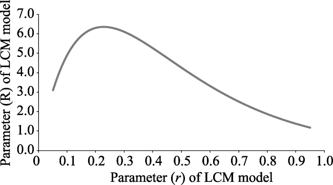
Figure 6 Relationship of R to r (LCM model) (α= [30, 210] mm/h, step=1; r=[0.05, 0.95], step= 0.001)

4 Conclusions

The SCS model and the LCM model are developed in the same period. They describe watershed runoff at the macroscopic scale, taking into account the relationship between total actual retention and total rainfall and having a certain similarity. In this study, by comparing the two runoff yield models using theoretical analyses and numerical simulations, we have found that: (1) the SCS model is a simple linear representation of the LCM model, and the LCM model reflects more significantly the nonlinearity of macro-runoff of the watershed. (2) There are strict mathematical relationships between LCM parameters (R, r) and SCS parameters (S). LCM parameters (R, r) can be determined using the research results of the SCS model parameters. (3) Parameters (R, r) of the LCM model can be easily measured by field experiments, while parameters (S) of the SCS model are difficult to obtain. Therefore, parameters (R, r) of the LCM model can provide the foundation for the SCS model. (4) SCS model has a linear relationship between reciprocal of the total actual retention and reciprocal of total rainfall during runoff period. The one-order terms of a Taylor series expansion of LCM model indicate the same relationship, which is worth further study.

The authors have declared that no competing interests exist.

1
Chen J Q, 1966. Estimation of Small Watershed Peak Discharge Resulting from Storm Rainfall, Report. Beijing: Hydro-Electric Publishing. (in Chinese)

2
Cronshey R, 1986. Urban hydrology for small watersheds. US Dept. of Agriculture, Soil Conservation Service, Engineering Division.

3
Hicks W I, 1944. A method of computing urban runoff.Trans. Amer. Soc. Civil Eng., 109: 1217-1253.

4
Liu Changming, Bai Peng, Gong Tonglianget al., 2013. Estimation of peak flow of an ungauged basin in Tibetan Plateau.South to North Water Transfers and Water Science & Technology, 11(1): 1-6. (in Chinese)

5
Liu Changming, Hong Baoxin, Zeng Mingxuanet al., 1965. The experimental research of the predicting relationship of storm runoff on Loess Plateau.Chinese Science Bulletin, 2(2): 158-160. (in Chinese)

6
Liu Changming, Wang Guangte, 1980. The estimation of small-watershed peak flows in China.Water Resources Research, 16(5): 881-886.

7
Liu Changming, Wang Zhonggen, Zheng Hongxinget al., 2008. Application study of HIMS system and custom model. Science in China (Series E: Technological Sciences), 38(3): 350-360. (in Chinese)

8
Liu Changming, Zheng Hongxing, Wang Zhonggenet al., 2010. The hydrological process of HIMS integrated simulation based on multi scale. Journal of Beijing Normal University (Natural Science Edition), 46(3): 268-273. (in Chinese)

9
Liu Changming, Zhong Junxiang, 1978. Preliminary analysis of effects of forest on runoff in Loess Plateau.Acta Geographica Sinica, 33(2): 112-126. (in Chinese)

10
Liang Kang, Liu Changming, Wang Zhonggenet al., 2012. Runoff simulation in the Heiyukou sub-basin of the Weihe River Basin and its responses to climate change based on HIMS.Yellow River, (10): 13-14. (in Chinese)

11
McCuen R H, 1982. A Guide to Hydrologic Analysis Using the SCS Methods. Prentice-Hall, Inc., 145p.

12
Mishra S K, Singh V P, 1999. Another look at the SCS-CN method.J. Hydrol. Eng., 4(3): 257-264.

13
Mishra S K, Singh V P, 2002a. SCS-CN-based hydrologic simulation package, Ch. 13. In: Singh V P, Frevert D K (eds). Mathematical Models in Small Watershed Hydrology and Applications, Water Resources Publications, P.O. Box 2841, Littleton, CO 80161, 391-464.

14
Mishra S K, Singh V P, 2002b. SCS-CN method. Part I: Derivation of SCS-CN based models.Acta Geophys. Pol., 50(3): 457-477

15
Mishra S K, Singh V P, 2003. Soil Conservation Service Curve Number (SCS-CN) Methodology. Dordrecht, The Netherlands: Kluwer.

16
Mishra S K, Singh V P, 2004a. Long-term hydrological simulation based on the soil conservation service curve number. Hydrol. Process, 18(7): 1291-1313

17
Mishra S K, Singh V P, 2004b. Validity and extension of the SCS-CN method for computing infiltration and rainfall-excess rates.Hydrol. Process., 18: 3323-3345.

18
Moore I D, Grayson R B, Ladson A R, 1991. Digital terrain modeling: A review of hydrological, geomorphological and biological applications.Hydrological Processes, 5(1): 3-30.

19
Patil J P, Sarangi A, Singh A Ket al., 2008. Evaluation of modified CN methods for watershed runoff estimation using a GIS-based interface.Biosystems Engineering, 100(1): 137-146.

20
Reyes M R, Green C H, Arnold J G, 2007. The soil and water assessment tool: Historical development, applications, and future research directions. Center for Agricultural and Rural Development, Iowa State University.

21
SCS, 1956. Hydrology. National Engineering Handbook, Supplement A, Section 4 Chapter 10, Soil Conservation Service. Washington: DC USDA.

22
SCS, 1971. Hydrology National Engineering Handbook. Section 4, Chapter 10, Soil Conservation Service. Washington, DC: USDA.

23
SCS, 1985. Hydrology. National Engineering Handbook, Supplement A, Section 4 Chapter 4, Soil Conservation Service. Washington, DC: USDA.

24
SCS, 2004

25
USDA, 1986. Urban hydrology for small watersheds. Tech release 55, Natural Resources Conservation Service, US Dept of Agriculture.

26
Wang Zhonggen, Zheng Hongxing, Liu Changming, 2005. Based distributed hydrological modeling system and its application modules.Progress in Geography, 24(6): 109-115. (in Chinese)

27
Wang Zhonggen, Zheng Hongxing, Liu Changminget al., 2004. Application study of the distributed hydrological model in the Yellow River typical watershed.Science in China (Series E: Science and Technology), 34(Suppl.I): 49-59. (in Chinese)

Outlines

/