Orginal Article

Start of vegetation growing season on the Tibetan Plateau inferred from multiple methods based on GIMMS and SPOT NDVI data

  • DING Mingjun , 1, 2 ,
  • LI Lanhui 1 ,
  • ZHANG Yili , 2, 3, * ,
  • SUN Xiaomin 2, 4 ,
  • LIU Linshan 2 ,
  • GAO Jungang 2 ,
  • WANG Zhaofeng 2 ,
  • LI Yingnian 5
Expand
  • 1. Key Lab of Poyang Lake Wetland and Watershed Research of Ministry of Education and School of Geography and Environment, Jiangxi Normal University, Nanchang 330022, China
  • 2. Key Laboratory of Land Surface Pattern and Simulation, Institute of Geographic Sciences and Natural Resources Research (IGSNRR), CAS, Beijing 100101, China
  • 3. CAS Center for Excellence in Tibetan Plateau Earth Sciences, Beijing 10101, China
  • 4. Key Laboratory of Ecosystem Network Observation and Modeling, IGSNRR, CAS, Beijing 100101, China
  • 5. Northwest Institute of Plateau Biology, CAS, Xining 810008, China;

*Corresponding author: Zhang Yili, Professor, E-mail:

Author: Ding Mingjun (1979-), PhD and Associate Professor, specialized in land-use/land-cover change and physical geography. E-mail:

Received date: 2014-08-18

  Accepted date: 2014-09-26

  Online published: 2015-02-15

Supported by

Strategic Priority Research Program of the Chinese Academy of Sciences, No.XDB03030500

National Natural Science Foundation of China, No.41201095;No.41171080;No.41371120

Copyright

Journal of Geographical Sciences, All Rights Reserved

Abstract

In this study, we have used four methods to investigate the start of the growing season (SGS) on the Tibetan Plateau (TP) from 1982 to 2012, using Normalized Difference Vegetation Index (NDVI) data obtained from Global Inventory Modeling and Mapping Studies (GIMSS, 1982-2006) and SPOT VEGETATION (SPOT-VGT, 1999-2012). SGS values estimated using the four methods show similar spatial patterns along latitudinal or altitudinal gradients, but with significant variations in the SGS dates. The largest discrepancies are mainly found in the regions with the highest or the lowest vegetation coverage. Between 1982 and 1998, the SGS values derived from the four methods all display an advancing trend, however, according to the more recent SPOT VGT data (1999-2012), there is no continuously advancing trend of SGS on the TP. Analysis of the correlation between the SGS values derived from GIMMS and SPOT between 1999 and 2006 demonstrates consistency in the tendency with regard both to the data sources and to the four analysis methods used. Compared with other methods, the greatest consistency between the in situ data and the SGS values retrieved is obtained with Method 3 (Threshold of NDVI ratio). To avoid error, in a vast region with diverse vegetation types and physical environments, it is critical to know the seasonal change characteristics of the different vegetation types, particularly in areas with sparse grassland or evergreen forest.

Cite this article

DING Mingjun , LI Lanhui , ZHANG Yili , SUN Xiaomin , LIU Linshan , GAO Jungang , WANG Zhaofeng , LI Yingnian . Start of vegetation growing season on the Tibetan Plateau inferred from multiple methods based on GIMMS and SPOT NDVI data[J]. Journal of Geographical Sciences, 2015 , 25(2) : 131 -148 . DOI: 10.1007/s11442-015-1158-y

1 Introduction

Plant phenology refers to the temporal pattern of seasonal leaf development and senescence (Ding et al., 2013). Environmental changes may alter vegetation phenology; and in turn, the altered phenology has a feed-back effect on surface-atmosphere exchanges of energy, water and carbon by controlling the leaf area index (LAI) (Niemand et al., 2005; Piao et al., 2007; Peñuelas et al., 2009; Richardson et al., 2009). As the best indicator for monitoring the influence of climate on vegetation, plant phenology has become the key target of global- change research (Menzel, 2002). Based on ground observation data, in the decade between 1991 and 2000 the spring phenological changes arrived earlier for most plants in Europe and North America (Fitter and Fitter, 2002; Menzel et al., 2006; Parmesan, 2007). Observational data for China also show that, from the 1980s onwards, the spring phenological changes arrived earlier in northern China (Zheng et al., 2002).
For some regions with harsh natural conditions, however, changes in vegetation phenology and their linkage to climate remain poorly understood, due to the lack of in situ observations of phenological data. This limits our ability to detect regional vegetation growth (Tang et al., 2009). Monitoring vegetation phenological changes at the regional and global levels could help to quantify the effects of climate change on terrestrial ecosystems. Therefore, time-series data from satellite remote sensing have been widely used for studying vegetation phenology at the landscape, regional and global levels (Myneni et al., 1997; Zhou et al., 2001; Jeong et al., 2011; Sobrino and Julien, 2011), given that there is a strong coincidence between satellite-derived metrics and ground-observed phenological characteristics (Reed et al., 1994). In recent years, several different methods have been developed to convert satellite signals to vegetation phenological phases (Moulin et al., 1997; Myneni et al., 1997; White et al., 2002; Zhang et al., 2003; Jeong et al., 2011; Kross et al., 2011).
These methods all involve two critical steps. In the first step, satellite-derived vegetation indices, such as the normalized difference vegetation index (NDVI), which are usually acquired over a period of half a month or 10 d, are expanded into time series that are suitable for phenological study, usually on a daily basis. Meanwhile, although the remote sensing data adopt the maximum-value composite (MVC) technique, effects at the sub-pixel level of contamination by residual clouds, long-term cloud haze or other negative influences cannot be removed. Therefore, further smoothing treatment is necessary, because these factors appear at random, causing the appearance of an unclear curvilinear change during the growing season. Through the use of these smoothing methods, noisy or abnormal points are filtered out based on particular mathematical rules, e.g., by using Gaussian filters (Jonsson and Eklundh, 2002), spline filters (White et al., 2009), Fourier filters (Roerink et al., 2000), and Savizky-Golay filters (Savitzky and Golay, 1964; White et al., 2009)). In the next step, critical thresholds for specific phenological events are determined from the reconstructed satellite signal time series by the application of specified rules (White et al., 2002; Zhang et al., 2003; Piao et al., 2009; White et al., 2009). However, individual methods vary in the rules that they adopt for expanding the time series and in determining the critical thresholds for specific phenological events. White et al. (2009) compared 10 commonly used methods for estimating the start-of-spring averaged by eco-region from the NDVI data derived from an advanced very high resolution radiometer (AVHRR) in North America and found that spatial phenological patterns derived from different methods often differed among eco-regions. Cong et al. (2012) has argued that it is critical to choose the “right” method for the “right” place in a vast region with diverse vegetation types and physical environments.
As the “third pole” of the world, the Tibetan Plateau (TP) has approximately 1,521,500 km2 of alpine grasslands (accounting for 59.15% of the total area of 2,572,400 km2 in the TP (Zhang et al., 2002)). Recent studies have indicated that the terrestrial ecosystems of the TP play a significant role in ensuring the ecological security of China and East Asia (Zhong et al., 2006; Sun et al., 2012; Zhang et al., 2014). Changes in the dates of start-of-spring and end-of autumn, and consequently the length of the growing season, are critical factors contributing to the observed carbon cycle dynamics, and they also influence stock-raising. Therefore, the achievement of an accurate understanding of the spatial patterns of the phenological changes on the TP, and of the forces driving them, appears especially important. Although the long-term observed phenological data are scarce for the TP due to its harsh physical environment, remote sensing data, including time-series NDVI data from Global Inventory Modeling and Mapping Studies (GIMMS), from SPOT VEGETATION (SPOT-VGT), and from the Moderate Resolution Imaging Spectroradiometer (MODIS), are available. Several recent studies using NDVI (GIMMS) have reported that the alpine steppes and meadows underwent start-of-the-growing-season (SGS) advancement before the end of the 1990s, but that there was then a delay in the SGS after the end of the 1990s, until 2006 (Yu et al., 2010; Piao et al., 2011). One study based on MODIS NDVI data showed that the alpine vegetation SGS advanced in most parts of the TP between 2001 and 2010 (Song et al., 2011). Two of the other studies based on SPOT-VGT NDVI data found an SGS delay between 1998 and 2003 and then an advancement between 2003 and 2009 (Shen, 2011; Ding et al., 2013). Zhang et al. (2013) have found that the GIMMS NDVI data for 2001-2006 differs substantially from the corresponding SPOT-VGT NDVI data and MODIS NDVI data and they have suggested that the GIMMS NDVI data may suffer from severe data-quality issues in most parts of the western plateau, so they thought that the SGS advanced continuously after the end of the 1990s based on SPOT-VGT NDVI data. Overall, studies concerning the trend in the SGS for alpine vegetation on the TP have shown varying results according to the different types of remote sensing data and methods that have been used. However, due to a lack of observed phenological data (Piao et al., 2011; Shen, 2011; Ding et al., 2013), there is as yet no study that has discussed the merits and shortcomings of each remote sensing method with respect to the TP.
In this study, we have applied four methods (Threshold of maximum relative change; Threshold of maximum relative change ratio; Threshold of NDVI ratio; and Maximum change of curvature), all of which are currently used in phenological studies on the TP, to investigate the SGS on the TP, using NDVI data from GIMMS and SPOT-VGT. We have focused on: (1) the spatial distribution and inter-annual change of the SGS; (2) the discrepancy in the SGS inferred from satellite data based on multiple models; and (3) in relation to vegetation phenology on the TP, which of the models is the most suitable based on the in situ observed phenological data, and in what respects are improvements necessary.

2 Data and methods

2.1 Dataset

We analyzed the vegetation phenology (SGS) on the TP by using two remote sensing datasets, GIMMS (1982-2006) and SPOT-VGT (1999-2012). NDVI, defined as the ratio of the difference between near-infrared reflectance and red visible reflectance to their sum, is an indicator of vegetation greenness (Myneni et al., 1997).
2.1.1 NDVI dataset from GIMMS
The GIMMS NDVI, the longest time-series NDVI dataset, covering the period from 1981 (July) to 2006, was provided by the Global Land Cover Facility of the University of Maryland (Tucker et al., 2005). The data were obtained from the Advanced Very High Resolution Radiometer (AVHRR) instrument onboard the National Oceanic and Atmospheric Administration (NOAA) satellite series 7, 9, 11, 14, 16, and 17. The GIMMS NDVI products, with a spatial resolution of 8 km, were compiled by merging segments (data strips) of a half-month period using the MVC method (Holben, 1986). These data had been calibrated for sensor shifts, and corrected to remove the effects of sensor degradation, satellite orbit drift, solar zenith angles and other factors, such as the effects of stratospheric aerosol loadings from the El Chichon and Mount Pinatubo eruptions in April 1984 and June 1991 (Zhou et al., 2001; Slayback et al., 2003).
2.1.2 NDVI dataset from SPOT-VGT
The SPOT-VGT NDVI, covering the period from 1998 (April) to 2012 and with a spatial resolution of 1 km, was derived from the vegetation instrument of the Système Pour l’Observation de la Terre (SPOT). Its temporal resolution was about 10 d, which therefore amounted to 36 composites in a single-year cycle. The dataset had been corrected to remove the effects of satellite shift and sensor degradation. Atmospheric contamination from water vapor, ozone and aerosols had also been corrected using a simplified method for atmospheric corrections (SMAC) (Rahman and Dedieu, 1994). In addition, the MVC for each 10-d interval was also applied in order to minimize further the non-vegetation effects (Holben, 1986; Maisongrande et al., 2004).
2.1.3 Preprocessing of NDVI data
Despite all the efforts to improve the data quality, the remaining atmospheric contamination in the NDVI dataset may still result in spurious variations in the vegetation indices (Chen et al., 2004) and may affect the detection of vegetation phenology. Therefore, in the present study, we used the smoothing method ‘Harmonic Analysis of Time Series’ (HANTS) in order to reduce further the potential noise. HANTS is a new method used in the analysis of plant phenology. It considers fully the plant growth cycle. Rebuilt time-series data based on this method can reflect the true periodic change properties of the curve (Roerink et al., 2000). The HANTS method was employed in the present work to carry out a smoothing treatment of the NDVI data obtained from GIMMS and SPOT-VGT. As a result of the HANTS treatment, two types of data were obtained: one comprised smoothed data having the same temporal resolution as the raw data; the other was the smoothed data with a temporal resolution of 1 day (Ding et al., 2013). Smoothed data were used only in Methods 1, 2 and 3 but not in Method 4. In this work, in order to eliminate the effects of bare soil, sparse vegetation and evergreen forest, the pixels needed to meet certain particular requirements. Based on the SPOT-NDVI in 2006, this study adopted the specific steps described in Ding et al. (2013) to process the data.

2.2 Methods

Currently, there are many methods which have been developed for retrieving SGS from seasonal NDVI data (Julien and Sobrino, 2009; Cong et al., 2012). However, an universally accepted definition of SGS does not exist (White et al., 2009). Recently, the techniques applied to vegetation phenological studies on the TP have included four methods, viz.: Threshold of maximum relative change, used by Piao et al., (2011) and Ding et al. (2013); Threshold of maximum relative change ratio, used by Zhang et al. (2013); Threshold of NDVI ratio, used by Yu et al. (2010 and 2012); and Maximum change of curvature, used by Shen et al. (2011). Meanwhile, these methods also are dominant ways and widely used in the other regions of the world in the study of the vegetation phenology. As the environment is unique, there is some faultiness to use these methods to derive SGS on the TP. In this study, we partially modified these methods.
2.2.1 Method 1 (Threshold of maximum relative change) (Figure 1a).
Based on the smoothed data with the same temporal resolution as the raw data (temporal resolution of 10 d or 15 d), we calculated the annual NDVI time series for each pixel and the relative NDVI change using the following formula (Piao et al., 2006):
where t is the time. We then used the corresponding NDVI(t) with the positive maximum ΔNDVI(t) as the NDVI threshold for the SGS date. Next, the second type of data obtained using HANTS (i.e., NDVI time-series data with a temporal resolution of 1 d) was used to determine the Julian day of the SGS. When the NDVI value of various pixels was larger than the SGS threshold within a specific time period, the day was regarded as the SGS.
2.2.2 Method 2 (Threshold of maximum relative change ratio) (Figure 1b).
Based on the smoothed data with the same temporal resolution as the raw data, we calculated the annual NDVI time-series curve for each pixel and the relative NDVI change ratio using the following formula (Zhang et al., 2013):
where t is the time. The subsequent steps were the same as in Method 1.
2.2.3 Method 3 (Threshold of NDVI ratio) (Figure 1c).
SGS values were modeled using the NDVI ratio method developed by White et al. (1997). Based on the smoothed data with the same temporal resolution as the raw data, we found the maximum and minimum NDVI values. Yu et al. (2010) evaluated the average NDVI curve over 24 years (GIMMS) and noted that the NDVI reached its minimum value in February and March. The average NDVI in these two months was thus used as NDVImin in place of the annual NDVI minimum, which might occur at the time of maximum snow cover. Then, based on the second type of data obtained through HANTS, we normalized all the NDVI values using (NDVImax - NDVImin). For SGS values, we selected an NDVI ratio threshold of 0.2. Using the thresholds, SGS values were estimated for each pixel of the study area for each year on record.
2.2.4 Method 4 (Maximum change of curvature) (Figure 1d).
To further reduce contamination by clouds, snow and ice, we applied a three-points-smooth method to each annual NDVI cycle, as described by Chen et al. (2000). We then divided the filtered time series into two phases by the time of annual maximum NDVI, and fitted them using a four-parameter logistic function (see also Zhang et al. (2003)):
where t is the Julian day, y(t) is the NDVI value at time t, a and b are fitting parameters, c+d is the maximum NDVI value, and d is the initial background NDVI value (Zhang et al., 2003). We then calculated the rate of change of the curvature (RCC, see Eq. (3) in Zhang et al. (2003)) of the fitted function. We then defined SGS as the time when RCC reached its first local maximum value (Zhang et al., 2003).
The retrieved SGS values based on the remote sensing data in this paper were validated by the observed phenological data from 19 agro-meteorological stations on the TP. As these stations are mainly located in the grasslands and meadows region, we supposed that the region where the station was located had homogeneous environment and the in situ observed data based on the station may represent the phenology of area around the station. In order to accord with the same spatial resolution as GIMMS and SPOT, the retrieved SGS values for the sites were averaged over a circular area with 8-km and 1-km radius centered each site for GIMMS and SPOT respectively. The retrieved SGS values for the sites were averaged over a circular area, with an 8-km and 1-km radius for the GIMMS and SPOT respectively, centered at each site.
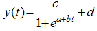
Figure 1 Schematic figures showing the methods of phenological detection. (a) Defining the NDVI threshold according to the NDVI relative change (NDVI(t + 1) - NDVI(t)) (Method 1). (b) Defining the NDVI threshold according to the NDVI relative change ratio ((NDVI(t + 1) - NDVI(t)) / NDVI(t)) (Method 2) in the NDVI seasonal cycle fitted by HANTS (with the same temporal resolution as the raw data), and then determining SGS by applying the NDVI threshold in each year’s NDVI seasonal cycle fitted by HANTS (with a temporal resolution of 1 d). (c) Determining the maximum and minimum NDVI values based on the smoothed data with the same temporal resolution as the raw data, and then normalizing all the NDVI values using (NDVImax - NDVImin) based on the smoothed data with a temporal resolution of 1 d and determining SGS by applying the NDVI ratio threshold (Method 3). (d) Based on the three-points-smooth data, modeling by the four-parameter logistic function, and then calculating the rate of change of the curvature and defining SGS as the time when RCC reached its first local maximum value (Method 4). For (a), (b) and (d), the change lines are shown in gray, while the smooth data are shown in black.

3 Results

3.1 Spatial distribution of vegetation SGS on the TP

In order to understand the spatial distribution of the SGS on the TP, we have analyzed the SGS of the general patterns and the different vegetation types, and also discussed the discrepancy in the SGS derived from satellite data based on multiple models.
3.1.1 General patterns
Using 25-year (1982-2006) GIMMS NDVI data and 13-year (1999-2012) SPOT NDVI data, we first show the spatial patterns of the multi-year average of SGS values retrieved using each method, the mean of the multi-year average of SGS obtained by each method and the standard deviation (SD) of the SGS values using the four methods (Figures 2 and 3). In general, the patterns are elevation- and longitude-dependent, and temperature, together with precipitation, is a key factor determining the spatial pattern. Vegetation growth in the center of the TP begins a little later than in the surrounding areas. Based on the average of results from the four methods above, for most pixels the SGS occurs between mid-April and late June. The SGS is delayed from east to west and it is also delayed with increasing elevation.
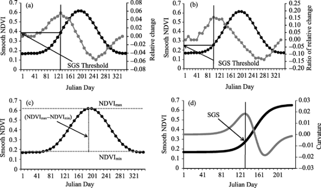
Figure 2 Spatial distribution of the vegetation SGS estimated from GIMMS NDVI data by the four methods described in the text. (a) Method 1; (b) Method 2; (c) Method 3; (d) Method 4; (e) Average of the four methods; and (f) SD of the four methods. The name of the physiographical regions are as follows: IB1 Golog-Nagqu high-cold shrub-meadow zone; IC1 Southern Qinghai high-cold meadow steppe zone; IC2 Qangtang high-cold steppe zone; ID1 Kunlun high-cold desert zone; IIAB1 Western Sichuan-eastern Tibet montane coniferous forest zone; IIC1 Southern Tibet montane shrub-steppe zone; IIC2 Eastern Qinghai-Qilian montane steppe zone; IID1 Ngari montane desert-steppe and desert zone; IID2 Qaidam montane desert zone; IID3 Northern slopes of Kunlun montane desert zone; OA1 Southern slopes of Himalaya montane evergreen broad-leaved forest zone (Zheng, 1996).
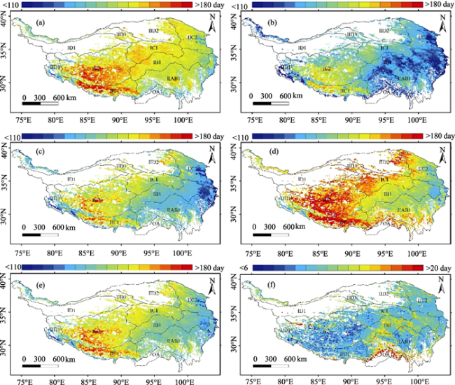
Figure 3 Spatial distribution of the vegetation SGS estimated from SPOT NDVI data by the four methods described in the text. (a) Method 1; (b) Method 2; (c) Method 3; (d) Method 4; (e) Average of the four methods; and (f) SD of the four methods. The others same as Figure 2.
Despite the similar spatial patterns revealed by the four methods using the GIMMS NDVI and the SPOT NDVI, there are still significant variations in the estimated SGS obtained using the different methods. Across this region, the range of SGS values estimated by the different methods varies mostly between 6 d and 20 d (GIMMS) and between 3 d and 21 d (SPOT). Comparing the results from the four methods, the SGS is usually earlier when measured by Method 2 or Method 3, especially Method 2. To test the methodological variation in SGS, we calculated the SD for each pixel of the estimated SGS obtained by the four different methods.
With regard to SGS, nearly 86.40% (GIMMS) or 46.37% (SPOT) of the total pixels show an SD of less than 10 d and nearly 11.73% (GIMMS) or 45.62% (SPOT) have an SD of between 10 d and 15 d, but on the other hand about 2.82% (GIMMS) or 8.01% (SPOT) of the total pixels show an SD of greater than 15 d. The largest discrepancies among the different methods are found mainly within the Golog-Nagqu high-cold shrub-meadow zone, the western Sichuan/eastern Tibet montane coniferous forest zone and the Eastern Qinghai-Qilian montane steppe zone (Zheng, 1996), all of which have comparatively high vegetation coverage for the TP. This implies that the regions with high coverage will exhibit larger discrepancies.
3.1.2 SGS of different vegetation types on the TP
Spatial variations of SGS values are also associated with the type of land cover (Yu et al., 2003; Zhang et al., 2004). Figure 4 shows a histogram of the SD of the SGS for each of the seven major vegetation types on the TP. Whereas most of the vegetation types have an SD of less than 15 d, significant variation exists within some vegetation types, particularly forest, scrub and alpine. The forests on the TP are mainly distributed within regions of low elevation around the plateau and consist of evergreen and deciduous forests. Although we have tried to remove the evergreen forests from our analysis, the pixels of forests contain some evergreen elements that may result in complicated NDVI curves; thus, phenological parameters estimated from remote sensing data may show remarkable discrepancies between the different methods. There also exists the problem of mixed pixels in regions with scrub cover; scrubs and meadows are often found together on the TP. The different phenological dates of the scrubs and meadows probably cause the complicated NDVI curves, and result in the discrepancies that are observed between the different methods. Alpine vegetation is mostly distributed in the regions of high elevation, where the vegetation coverage is comparatively low. In summary, the effect of the factors mentioned above is that the vegetation coverage often leads to remarkable discrepancies between the SGS values obtained by different methods.
Figure 5 shows a histogram of the SGS distribution for the entire region and for each of the seven major vegetation types on the TP. Although, overall, SGS mainly occurs in May and early June, for each vegetation type, there exists significant variation in SGS when it is measured using different methods. Thus SGS based on Method 2 is the earliest (occurring before Julian day 150 for most vegetation types), SGS determinations based on Methods 1 and 3 are intermediate and SGS measured by Method 4 is the latest (occurring after Julian day 130 for most vegetation types). As shown in Figure 5, areas with a high coverage of vegetation (forests, scrubs and crops) show an earlier SGS than areas with low vegetation coverage (alpine areas, deserts and grasslands).
The results indicate that the vegetation coverage significantly influences the SGS derived using the different methods. Clearly, it is important to pay attention to the vegetation types with high or low coverage when studying the vegetation phenology on the TP using different remote sensing techniques. Cong et al. (2012; 2013) also thought that the large inter-method variance was notably observed in the agriculture cropland, the arid and semiarid vegetation type, which is according with our results.

3.2 Inter-annual phenological changes on the TP

In the present study, as shown in Figure 6, from 1982 until 1998 the SGS values derived using the four methods all display an advancing trend. The variation amplitudes are between 3.1 d/10a and 5.0 d/10a, but the significance levels are not high, due to the large size of the fluctuations. The advancing trend is mainly controlled by the highest value in 1982 and the lowest value in 1998. From 1998 until 2003, SGS values show a delaying trend, and this is then followed by an advancing trend from 2003 until 2008. After 2008, SGS values exhibit a delaying trend. Generally, according to SPOT (1999-2012), there is no continuously advancing trend in SGS on the TP. We have also analyzed the correlation between the SGS values derived from GIMMS and SPOT for the years 1999-2006 using the four methods and have found that the correlation coefficients based on the four methods are 0.91 (P=0.002), 0.92 (P=0.001), 0.90 (P=0.002) and 0.85 (P=0.008), respectively. From the analysis above, though the values for SGS derived from the four methods or two remote sensing datasets exhibit discrepancies, the trend of the change maintains consistency.
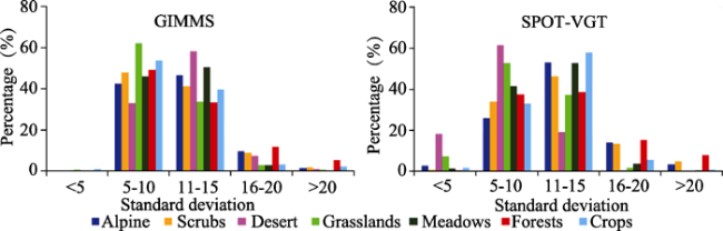
Figure 4 Histograms of the SDs of vegetation SGS values, for different vegetation types
Figure 5 Histograms of SGS values for different vegetation types, as determined by four methods
Previous studies using GIMMS NDVI have shown that a prominent reversal in the vegetation SGS occurred on the TP at the end of the 1990s, with a significant trend towards advanced SGS from 1982 to 1998 and then a trend towards a delayed SGS from 1998 to 2006 (Yu et al., 2010; Piao et al., 2011; Ding et al., 2013). Zhang et al. (2013) have stated that the GIMMS NDVI data-quality problem that occurred in spring during the years
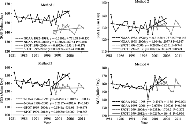
Figure 6 Inter-annual variations of vegetation SGS on the TP from 1982 to 2012; GIMMS data are shown in black and SPOT data are shown in gray
2001-2006 in most parts of the western TP is responsible for the spring phenological delay on the TP between 1998 and 2006; based on the SPOT and MODIS data, they have thought the SGS had been in advance from 1982 to 2011. On the other hand, based on SPOT-VGT data, Shen et al. (2013) have concluded that there is no evidence for a continuously advancing trend of SGS on the TP during the period from 1999 to 2012. Our results are in accordance with the results of Shen et al. (2013) but contradictory to those of Zhang et al. (2013).

3.3 Evaluation using in situ observed data of the SGS retrieved by the use of different models

The results and discussions above demonstrate that there are significant differences in the SGS values derived using the different methods. Here, we compare the four methods further and evaluate their suitability for the TP. The SGS values obtained by the application of the four methods in this paper have been validated using the observed phenological data obtained from 19 agro-meteorological stations on the TP.
Figure 7 shows a comparison between the in situ observed data and our retrieved results obtained using GIMMS data. For all sites, there are different levels of consistency between the observed and the retrieved SGS values, according to which of the four methods has been used. Although the mean absolute error (MAE) and the root-mean-square error (RMSE) for Method 2 are somewhat lower than for the other three methods, the R value is very low and does not qualify as significant (P < 0.01). For Method 3, the MAE and the RMSE are slightly larger than for Method 2; however, its R value is also larger and exceeds the significance level (P < 0.01).
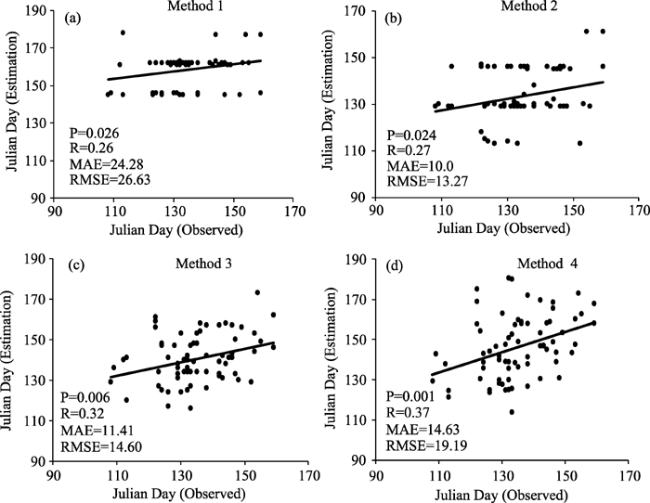
Figure 7 Comparison between SGS estimated by the four methods described in the text (using GIMMS data) and the observed SGS data from 19 agro-meteorological stations on the TP
Figure 8 shows the corresponding comparison using SPOT-VGT data. Again, for all sites, there are different levels of consistency between the observed and the calculated SGS values, according to which of the four methods has been used. Although for Method 1 the MAE and the RMSE are somewhat lower than for the other methods, R is very low; for Method 3, although the MAE and RMSE values are slightly larger than for Method 1, R is large and is significant.
For Methods 1 and 2, because the NDVI thresholds are confirmed based on the original time resolution (GIMMS with a half-month period and SPOT with a 10-d period), the SGS values are affected by the original time resolution, even though they are derived from the smoothed data, which has a single-day resolution. As shown in Figures 7 and 8, the SGS values derived using Method 1 or Method 2 show similar dates. The SGS values based on Methods 3 and 4 are derived from the smoothed data with single-day resolution directly, and the distribution of the SGS dates is relatively reasonable and never influenced by the original time resolution. Method 4, however, defines SGS as the time when RCC reaches its first local maximum value, which will result in an earlier date for SGS.
At present, there are many researches focusing on SGS retrieved using remote sensing on the TP (Piao et al., 2011; Shen et al., 2011; Song et al., 2011; Ding et al., 2013; Zhang et al., 2013), but none of them has evaluation using in situ observed data in detail. Based on the analysis of evaluation above, we consider that Method 3 is more applicable than the other methods comparatively. However, the in situ observed data are mainly distributed in the grasslands and meadows. Such a lack of in situ observation data in the other vegetation types still limits our understanding of the adoption of the methods used to retrieve vegetation phenology based on remote sensing on the TP.
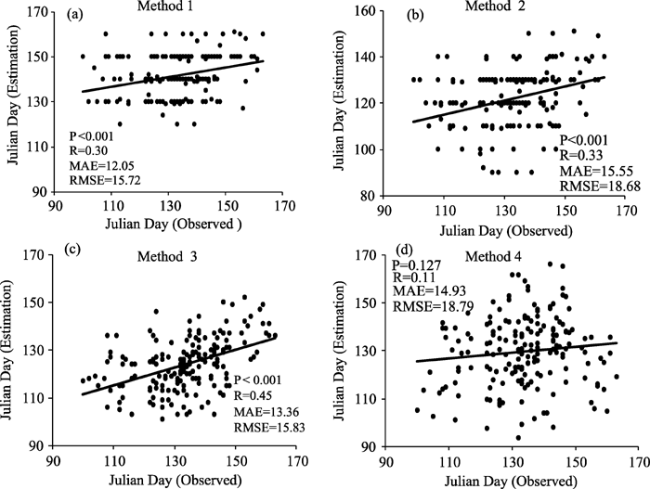
Figure 8 Comparison between SGS estimated by the four methods described in the text (using SPOT data) and the observed SGS data from 19 agro-meteorological stations on the TP

4 Discussion

Satellite-derived greenness vegetation indices provide a method of acquiring spatio-temporal information about vegetation phenology and have thus been widely used to assess the influences of climatic changes on vegetation, especially in regions where field observations are scarce (Piao et al., 2006; Yu et al., 2010; 2012; Ding et al., 2013). However, satellite-derived phenology data should be viewed with caution, because vegetation indices are easily contaminated by adverse meteorological conditions and background changes, such as cloud cover, bare soil and snow cover, which often make the signal weak (Shen et al., 2013). Though the remote sensing data have already been processed to lower the noise, sometimes these occasional interferences still result in vegetation indices less than the actual value. As shown in Figure 9, there are some fluctuations within the yearly NDVI curves. As is well known, in regions with a natural vegetation distribution, the real NDVI curve never displays a sudden decrease, which often causes errors in satellite-derived phenological data. Therefore, smoothing methods are widely used for the extraction of phenological information. We sampled two sites, using raw and smooth data from GIMMS in 2006, in order to explore the effects of the fluctuation on the phenological information that was extracted. At Qilian, the vegetation SGS values that were extracted from the raw data based on Methods 1, 2 and 3 were on the 48th, 48th and 158th Julian days, respectively, whereas those that were extracted from the smoothed data were on the 158th, 142th and 158th Julian days, respectively. At Qingshuihe, the vegetation SGS values extracted from the raw data were on the 158th, 142th and 158th Julian days, respectively, whereas those extracted from the smoothed data were on the 142th, 111th and 127th Julian days, respectively.
From the results above, it is clear that the smoothing method can eliminate the very obvious errors caused by the fluctuations. Shen et al. (2013) considered that the non-growing-season NDVI values should remain constant throughout different years and adopt a procedure (not mentioned in their paper) to eliminate the differences in the non-growing-season NDVI values between different years. They then found that there was no change in SGS in 2009-2011 compared to 1998-2000, although they also used smoothing method. Sometimes, however, the smoothing method may elevate the growth curve, particularly at the time when the SGS appears, and it probably makes the SGS advanced (Figure 9) and creates errors. Though there are many smoothing methods that have been used to retrieve vegetation phenological information, the merits and defects of these methods require more in-depth discussion.
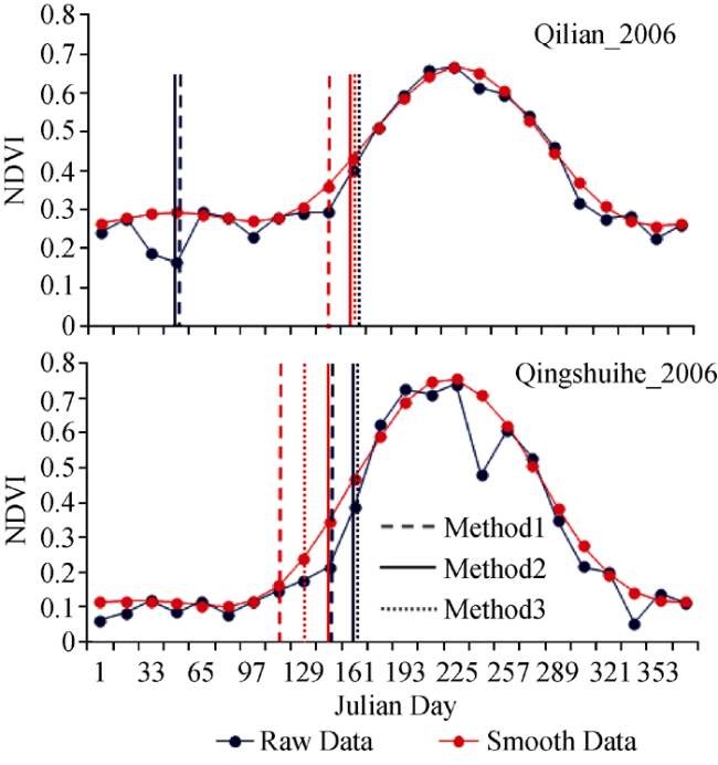
Figure 9 Vegetation growth curves at two sample sites in 2006 (Qilian and Qingshuihe) based on GIMMS data. The blue and red straight lines show the extracted vegetation phenological information based on the raw and smoothed data, respectively. The NDVI values were averaged within a circular area, with an 8-km radius, centered at each site. The phenological information is calculated using Methods 1, 2 and 3.
Many studies that used Method 1 (Piao et al., 2011) and Method 2 (Zhang et al., 2013) to retrieve vegetation phenological information on the TP first calculated the multi-year average NDVI time-series curve from 1982 to 2006 and then used the corresponding NDVI(t) with the maximum ΔNDVI or ΔNDVIratio as the NDVI threshold for the SGS date (details in section 2.2). However, using multi-year averaging to determine the NDVI threshold is not suitable, as shown in Figure 10, due to the time of the annual maximum NDVIratio being different in different years, which results in different thresholds. Using the threshold, a multi-year average threshold can lead to an earlier SGS when the yearly maximum NDVI is higher and a later SGS when the yearly maximum NDVI is lower. Shen et al. (2013) also considered that Methods 1 and 2 assumed that the non-growing-season NDVI values remained constant over different years and that sophisticated reprocessing of the non-growing-season NDVI was therefore required; otherwise, the retrieved SGS would be negatively biased by the increase in the non-growing-season NDVI. For this reason, we have used the corresponding annual NDVI(t) with the maximum △NDVI or △NDVIratio instead of the multi-year average as the NDVI threshold for the annual SGS date.
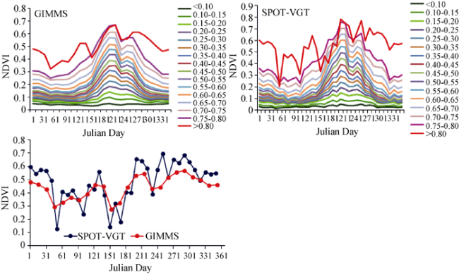
Figure 10 Schematic diagram indicating different yearly NDVI curves (GIMMS) in different years, which probably biases the derived SGS
All the methods used for phenological estimations based on remote sensing have assumed that the natural vegetation growth curve includes four phases within a single year: non-variation, increase, decrease and non-variation. Nevertheless, in areas with sparse vegetation and evergreen forests, the NDVI is influenced by adverse meteorological conditions, background changes and other factors; the consequence of this is that the yearly NDVI curve never displays according to this assumption, as shown in Figure 11. It causes serious errors in extracting vegetation phenological information over large areas, especially in the northern, western and southeastern parts of the TP. For example, as shown in Figure 2 of Yu et al. (2010) [and also in the figures of Yu et al. (2012)] and in Figure 3 of Zhang et al. (2013), there are errors of phenology in the northern and southeastern TP. In order to minimize the impact of soil variations in bare and sparsely vegetated regions, many researchers adopt particular criteria so as to erase such areas. Piao et al. (2011) and Zhang et al. (2013) only consider pixels with an average NDVI from April to October larger than 0.1, similar to the criterion of Zhou et al. (2001). In addition to the criterion above, other researchers introduce several other rules (Shen et al., 2011; Ding et al., 2013). Moreover, in order to eliminate the impact of evergreen forests on the results, land-use and land-cover maps are used in many studies, despite the uncertainties of such maps. Therefore, in order to eliminate the effects upon the data of bare soil, sparse vegetation and evergreen forests, we conclude that only pixels that simultaneously meet the following criteria are suitable to be used in phenological analysis on the TP. These criteria are as follows: 1) the average value of NDVI in April-September shall be more than 0.10; 2) the maximum value of annual NDVI shall exceed 0.15; 3) the annual maximum value shall occur between July and September; and 4) the average value of NDVI in winter shall be less than 0.4 (Ding et al., 2013; Shen et al., 2011).
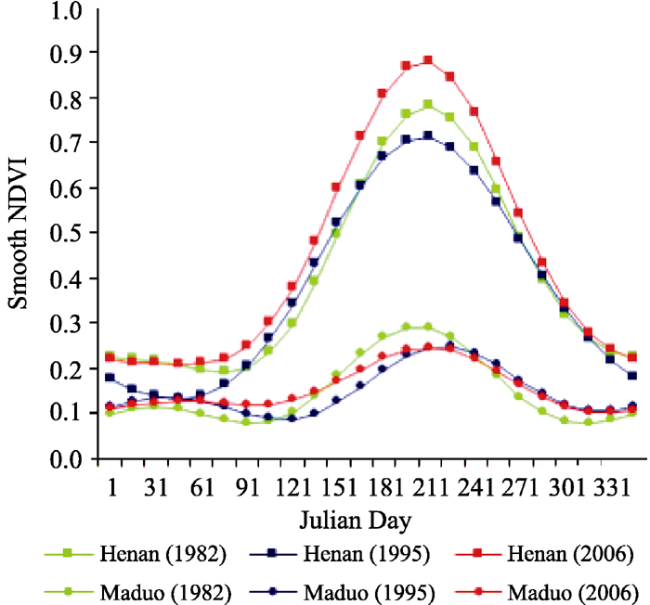
Figure 11 Vegetation growth curves in regions with different NDVI grades (a, b), and on the southern slopes of the Himalaya montane evergreen broad-leaved forest zone (c), based on the mean NDVI, over many years, of the GIMSS (1982-2006) and SPOT-VGT (1999-2012) data
In this study, based on the GIMMS and SPOT NDVI data, we have focused on the discrepancy in the SGS inferred from multiple methods and the applicability of methods. Besides, we have also discussed the improvements necessary of the methods. However, previous studies demonstrated that the different sensor products can also lead to discrepancy in the SGS except for methods, because there exists inconsistency among them (Hogda et al., 2013; Jiang et al., 2013; Zhang et al., 2013), which can be seen from Figures 2, 3 and 6 in the study as well. Though we have analyzed the correlation between the SGS derived from the GIMMS and SPOT, the same study period is relatively short, which limited our understanding the discrepancy between the two types of remote sensing data. Nevertheless, currently, there are many studies which used different remote sensing products to analyze vegetation phenology (Myneni et al., 1997; Zhou et al., 2001; Jeong et al., 2011; Sobrino and Julien, 2011), therefore, the assessment of the discrepancy among the SGS derived from different remote sensing data is very important and necessary.

5 Conclusions

In this paper, we have studied the SGS phenology on the TP using four methods based on GIMMS and SPOT NDVI data.
(1) For all four methods, the SGS was delayed increasingly from east to west and also with increasing elevation. However, discrepancies exist between the SGS dates estimated using the four methods. Generally, Method 4 produces the latest estimate of SGS, whereas Method 2 produces the earliest. The methods produce differences in SGS estimates that vary across different vegetation types and regions within the TP. The largest discrepancies amongst the four methods are associated mainly with the regions with the highest or lowest vegetation coverage, such as forests, areas of scrub, agricultural areas and alpine regions. Vegetation coverage plays an important role in all the different methods. More attention needs to be paid to vegetation types with high or low coverage when studying vegetation phenology on the TP using the various remote sensing techniques.
(2) Between 1982 and 1998, the SGS values derived from the four methods all display an advancing trend, with a variation in amplitude between 3.1 d/10a and 5.0 d/10a; however, the significance levels are not high, due to the large size of the fluctuations. The advancing trend is mainly determined by the highest value, in 1982, and the lowest value, in 1998. From 1998 to 2003, SGS values show a delaying trend, and then display an advancing trend from 2003 to 2008. From 2008 onwards, the SGS values exhibit a delaying trend. Generally, according to the SPOT data, there is no continuously advancing trend in SGS on the TP from 1999 to 2012. Moreover, we have analyzed the correlation between the SGS values derived from the GIMMS and SPOT data for the period between 1999 and 2006; the four analysis methods produce a consistent trend with respect to the change in SGS.
(3) Regarding the comparison with the observed phenological data obtained from 19 agro-meteorological stations on the TP, we consider that Method 3 is more applicable than the other methods comparatively.
However, the in situ observed data are mainly distributed in the grasslands and meadows. Such a lack of in situ observation data in the other vegetation types still limits our understanding of the adoption of the methods used to retrieve vegetation phenology based on remote sensing on the TP. Overall, explicit historical data from both satellite and in situ observations are undoubtedly required to validate and correct the results presented here.

The authors have declared that no competing interests exist.

1
Chen J, Jönsson P, Tamura Met al., 2004. A simple method for reconstructing a high-quality NDVI time-series data set based on the Savitzky-Golay filter.Remote Sensing of Environment, 91(3): 332-344.

2
Chen X Q, Tan Z J, Schwartz M Det al., 2000. Determining the growing season of land vegetation on the basis of plant phenology and satellite data in northern China.International Journal of Biometeorology, 44(2): 97-101.

3
Cong N, Piao S L, Chen A Pet al., 2012. Spring vegetation green-up date in China inferred from SPOT NDVI data: A multiple model analysis.Agricultural and Forest Meteorology, 165: 104-113.

4
Cong N, Wang T, Nan H Jet al., 2013. Changes in satellite-derived spring vegetation green-up date and its linkage to climate in China from 1982 to 2010: A multi-method analysis.Global Change Biology, 19(3): 881-891.

5
Ding M J, Zhang Y L, Sun X Met al., 2013. Spatiotemporal variation in alpine grassland phenology in the Qinghai-Tibetan Plateau from 1999 to 2009.Chinese Science Bulletin, 58(3): 396-405.

6
Fitter A H, Fitter R S R, 2002. Rapid changes in flowering time in British plants.Science, 296(5573): 1689-1691.

7
Hogda K A, Tommervik H, Karlsen S R, 2013. Trends in the start of the growing season in Fennoscandia 1982-2011.Remote Sensing, 5(9): 4304-4318.

8
Holben B N, 1986. Characteristics of maximum-value composite images from temporal AVHRR data.International Journal of Remote Sensing, 7(11): 1417-1434.

9
Jeong S J, Ho C H, Gim H Jet al., 2011. Phenology shifts at start vs. end of growing season in temperate vegetation over the Northern Hemisphere for the period 1982-2008.Global Change Biology, 17(7): 2385-2399.

10
Jiang N, Zhu W Q, Zheng Z Tet al., 2013. A comparative analysis between GIMSS NDVIg and NDVI3g for monitoring vegetation activity change in the Northern Hemisphere during 1982-2008.Remote Sensing, 5(8): 4031-4044.

11
Jonsson P, Eklundh L, 2002. Seasonality extraction by function fitting to time-series of satellite sensor data.IEEE Transactions on Geoscience and Remote Sensing, 40(8): 1824-1832.

12
Julien Y, Sobrino J A, 2009. Global land surface phenology trends from GIMMS database.International Journal of Remote Sensing, 30(13): 3495-3513.

13
Kross A, Fernandes R, Seaquist Jet al., 2011. The effect of the temporal resolution of NDVI data on season onset dates and trends across Canadian broadleaf forests.Remote Sensing of Environment, 115(6): 1564-1575.

14
Maisongrande P, Duchemin B, Dedieu G, 2004. VEGETATION/SPOT: An operational mission for the Earth monitoring; presentation of new standard products.International Journal of Remote Sensing, 25(1): 9-14.

15
Menzel A, 2002. Phenology: Its importance to the global change community.Climatic Change, 54(4): 379-385.

16
Menzel A, Sparks T H, Estrella Net al., 2006. European phenological response to climate change matches the warming pattern.Global Change Biology, 12(10): 1969-1976.

17
Moulin S, Kergoat L, Viovy Net al., 1997. Global-scale assessment of vegetation phenology using NOAA/AVHRR satellite measurements.Journal of Climate, 10(6): 1154-1170.

18
Myneni R B, Keeling C D, Tucker C Jet al., 1997. Increased plant growth in the northern high latitudes from 1981 to 1991.Nature, 386(6626): 698-702.

19
Niemand C, Kostner B, Prasse Het al., 2005. Relating tree phenology with annual carbon fluxes at Tharandt forest.Meteorologische Zeitschrift, 14(2): 197-202.

20
Parmesan C, 2007. Influences of species, latitudes and methodologies on estimates of phenological response to global warming.Global Change Biology, 13(9): 1860-1872.

21
Peñuelas J, Rutishauser T, Filella I, 2009. Phenology feedbacks on climate change.Science, 324(5929): 887.

22
Piao S L, Cui M D, Chen A Pet al., 2011. Altitude and temperature dependence of change in the spring vegetation green-up date from 1982 to 2006 in the Qinghai-Xizang Plateau.Agricultural and Forest Meteorology, 151(12): 1599-1608.

23
Piao S L, Fang J Y, Ciais Pet al., 2009. The carbon balance of terrestrial ecosystems in China.Nature, 458(7241): 1009-1013.

24
Piao S L, Fang J Y, Zhou L Met al., 2006. Variations in satellite-derived phenology in China’s temperate vegetation.Global Change Biology, 12(4): 672-685.

25
Piao S L, Friedlingstein P, Ciais Pet al., 2007. Growing season extension and its impact on terrestrial carbon cycle in the Northern Hemisphere over the past 2 decades. Global Biogeochemical Cycles, 21(3): GB3018.

26
Rahman H, Dedieu G, 1994. SMAC: A simplified method for the atmospheric correction of satellite measurements in the solar spectrum.Remote Sensing, 15(1): 123-143.

27
Reed B C, Brown J F, VanderZee Det al., 1994. Measuring phenological variability from satellite imagery.Journal of Vegetation Science, 5(5): 703-714.

28
Richardson A D, Hollinger D Y, Dail D Bet al., 2009. Influence of spring phenology on seasonal and annual carbon balance in two contrasting New England forests.Tree Physiology, 29(3): 321-331.

29
Roerink G J, Menenti M, Verhoef W, 2000. Reconstructing cloud-free NDVI composites using Fourier analysis of time series.International Journal of Remote Sensing, 21(9): 1911-1917.

30
Savitzky A, Golay M J E, 1964. Smoothing and differentiation of data by simplified least squares procedures.Analytical Chemistry, 36(8): 1627-1639.

31
Shen M G, 2011. Spring phenology was not consistently related to winter warming on the Tibetan Plateau.Proceedings of the National Academy of Sciences, 108(19): E91-E92.

32
Shen M G, Sun Z Z, Wang S Pet al., 2013. No evidence of continuously advanced green-up dates in the Tibetan Plateau over the last decade.Proceedings of the National Academy of Sciences, 110(26): E2329.

33
Shen M G, Tang Y H, Chen Jet al., 2011. Influences of temperature and precipitation before the growing season on spring phenology in grasslands of the central and eastern Qinghai-Tibetan Plateau.Agricultural and Forest Meteorology, 151(12): 1711-1722.

34
Slayback D A, Pinzon J E, Los S Oet al., 2003. Northern hemisphere photosynthetic trends 1982-99.Global Change Biology, 9(1): 1-15.

35
Sobrino J A, Julien Y, 2011. Global trends in NDVI-derived parameters obtained from GIMMS data.International Journal of Remote Sensing, 32(15): 4267-4279.

36
Song C Q, You S C, Ke L Het al., 2011. Spatio-temporal variation of vegetation phenology in the Northern Tibetan Plateau as detected by MODIS remote sensing.Chinese Journal of Plant Ecology, 35(8): 853-863. (in Chinese)

37
Sun H L, Zheng D, Yao T Det al., 2012. Protection and construction of the national ecological security shelter zone on Tibetan Plateau.Acta Geographica Sinica, 67(1): 3-12. (in Chinese)

38
Tang Y H, Wan S Q, He J Set al., 2009. Foreword to the special issue: Looking into the impacts of global warming from the roof of the world.Journal of Plant Ecology, 2(4): 169-171.

39
Tucker C J, Pinzon J E, Brown M Eet al., 2005. An extended AVHRR 8-km NDVI dataset compatible with MODIS and SPOT vegetation NDVI data.International Journal of Remote Sensing, 26(20): 4485-4498.

40
White M A, De Beurs K M, Didan Ket al., 2009. Inter-comparison, interpretation, and assessment of spring phenology in North America estimated from remote sensing for 1982-2006.Global Change Biology, 15(10): 2335-2359.

41
White M A, Nemani R R, Thornton P Eet al., 2002. Satellite evidence of phenological differences between urbanized and rural areas of the eastern United States deciduous broadleaf forest.Ecosystems, 5(3): 260-273.

42
White M A, Thornton P E, Running S W, 1997. A continental phenology model for monitoring vegetation responses to inter-annual climatic variability.Global Biogeochemical Cycles, 11(2): 217-234.

43
Yu F F, Price K P, Ellis Jet al., 2003. Response of seasonal vegetation development to climatic variations in eastern central Asia.Remote Sensing of Environment, 87(1): 42-54.

44
Yu H Y, Luedeling E, Xu J C, 2010. Winter and spring warming result in delayed spring phenology on the Tibetan Plateau.Proceedings of the National Academy of Sciences, 107(51): 22151-22156.

45
Yu H Y, Xu J C, Okuto Eet al., 2012. Seasonal response of grasslands to climate change on the Tibetan Plateau.PloS One, 7(11): e49230.

46
Zhang G L, Zhang Y J, Dong J Wet al., 2013. Green-up dates in the Tibetan Plateau have continuously advanced from 1982 to 2011.Proceedings of the National Academy of Sciences, 110(11): 4309-4314.

47
Zhang X Y, Friedl M A, Schaaf C Bet al., 2003. Monitoring vegetation phenology using MODIS.Remote Sensing of Environment, 84(3): 471-475.

48
Zhang X Y, Friedl M A, Schaaf C Bet al., 2004. Climate controls on vegetation phenological patterns in northern mid‐and high latitudes inferred from MODIS data.Global Change Biology, 10(7): 1133-1145.

49
Zhang Y L, Li B Y, Zheng D, 2002. A discussion on the boundary and area of the Tibetan Plateau in China.Geographical Research, 21(1): 1-8. (in Chinese)

50
Zhang Y L, Qi W, Zhou C Pet al., 2014. Spatial and temporal variability in the net primary production of alpine grassland on the Tibetan Plateau since 1982.Journal of Geographical Sciences, 24(2): 269-287.

51
Zheng D, 1996. The system of physico-geographical regions of the Qinghai-Xizang (Tibet) Plateau. Science in China (Series D), 39(4): 410-417.

52
Zheng J Y, Ge Q S, Hao Z X, 2002. Impacts of climate warming on plants phenophases in China for the last 40 years.Chinese Science Bulletin, 47(21): 1826-1831.

53
Zhong X H, Liu S Z, Wang X Det al., 2006. A research on the protection and construction of the State Ecological Safe Shelter Zone on the Tibet Plateau.Journal of Mountain Science, 24(2): 129-136. (in Chinese)

54
Zhou L, Tucker C J, Kaufmann R Ket al., 2001. Variations in northern vegetation activity inferred from satellite data of vegetation index during 1981 to 1999.Journal of Geophysical Research: Atmospheres (1984-2012), 106(D17): 20069-20083.

Outlines

/