
Journal of Geographical Sciences >
Reconstructing pre-erosion topography using spatial interpolation techniques: A validation-based approach
Author: Rafaello Bergonse, E-mail:rafaellobergonse@gmail.com
Received date: 2013-06-05
Accepted date: 2014-04-20
Online published: 2015-02-15
Copyright
Understanding the topographic context preceding the development of erosive landforms is of major relevance in geomorphic research, as topography is an important factor on both water and mass movement-related erosion, and knowledge of the original surface is a condition for quantifying the volume of eroded material. Although any reconstruction implies assuming that the resulting surface reflects the original topography, past works have been dominated by linear interpolation methods, incapable of generating curved surfaces in areas with no data or values outside the range of variation of inputs. In spite of these limitations, impossibility of validation has led to the assumption of surface representativity never being challenged. In this paper, a validation-based method is applied in order to define the optimal interpolation technique for reconstructing pre-erosion topography in a given study area. In spite of the absence of the original surface, different techniques can be nonetheless evaluated by quantifying their capacity to reproduce known topography in unincised locations within the same geomorphic contexts of existing erosive landforms. A linear method (Triangulated Irregular Network, TIN) and 23 parameterizations of three distinct Spline interpolation techniques were compared using 50 test areas in a context of research on large gully dynamics in the South of Portugal. Results show that almost all Spline methods produced smaller errors than the TIN, and that the latter produced a mean absolute error 61.4% higher than the best Spline method, clearly establishing both the better adjustment of Splines to the geomorphic context considered and the limitations of linear approaches. The proposed method can easily be applied to different interpolation techniques and topographic contexts, enabling better calculations of eroded volumes and denudation rates as well as the investigation of controls by antecedent topographic form over erosive processes.
Rafaello BERGONSE , Eusébio REIS . Reconstructing pre-erosion topography using spatial interpolation techniques: A validation-based approach[J]. Journal of Geographical Sciences, 2015 , 25(2) : 196 -210 . DOI: 10.1007/s11442-015-1162-2
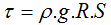
Table 1 Contexts and methodologies of some published pre-erosion surface reconstructions |
| Author | Purpose of reconstruction | Interpolation method |
|---|---|---|
| Wells and Gutiérrez (1982) | Estimation of eroded volumes and combination of results with current mean erosion rates in order to date badland initiation | Undefined |
| Daba et al. (2003) | Estimation of eroded volume in a large gully system for two different dates; comparison of results in order to quantify temporal evolution | Undefined1 |
| Alexander et al. (2008) | Understanding the geomorphic evolution of a badland site from a set of remnant surfaces, and estimating rates of denudation | Linear interpolation (Triangulated Irregular Networks) |
| Perroy et al. (2010) | Estimating volumetric soil loss from a set of gully channels | Linear interpolation (grid based) |
| Buccolini et al. (2012) | Estimating the volume eroded by a set of gully systems (calanchi), and relating pre-erosion topography to gully system properties | Linear interpolation (manual2) |
1 Authors used the SCOP (Stuttgard Contour Program) software to interpolate surfaces, but the specific method is not identified.2 Straight contour lines were drawn connecting points with the same height on both sides of the watershed of each calanco. |
Figure 1 The two study basins in the context of the lower Tagus. The set of 90 gullies and gully complexes subjected to pre-erosion surface reconstruction is identified |
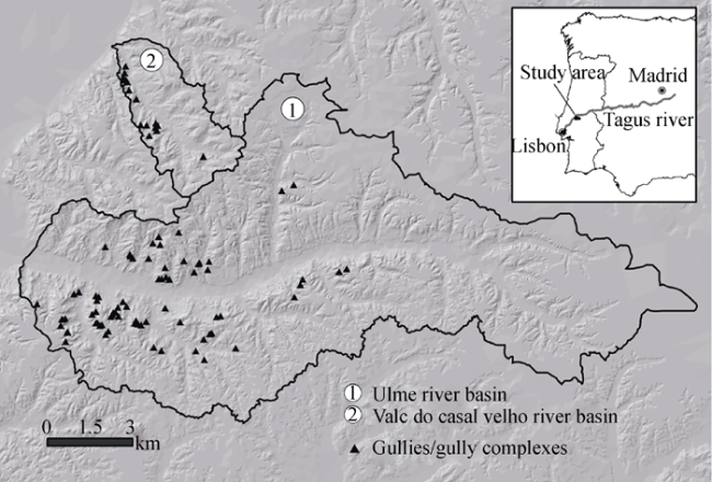
Figure 2 A large gully complex in the Ulme river basin. Walls show signs of active retreat (note deposits at the base and Quercus suber with root system completely exposed), contrasting with bottom colonized by vegetation |
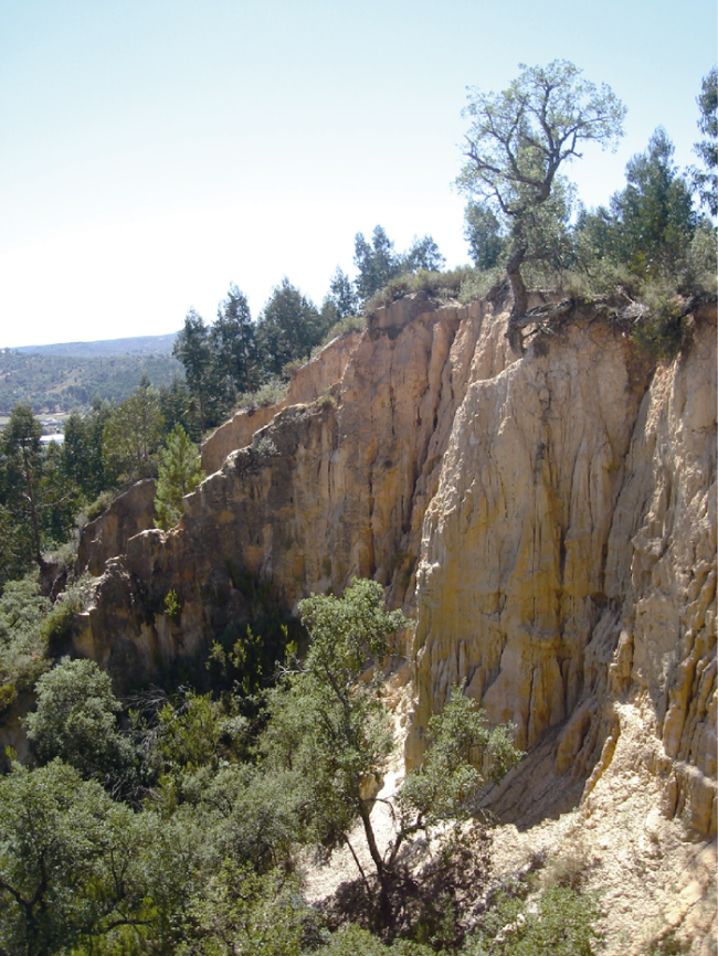
Figure 3 A schematic outline of the adopted methodology |
Table 2 General properties of the most common commercially available exact spatial interpolation methods |
| Method | General features | Smoothing | Proximity | Geostatistical assumptions |
|---|---|---|---|---|
| Linear interpolation | May be based on a previous Delaunay triangulation, with the value for each cell being defined by the linear surface of the triangle it overlays (e.g. Surfer 101, ArcGIS 9.1). In other cases, estimations are obtained simply as a function of the nearest known values and the respective distances (e.g. IDRISI Andes2: Eastman, 2006) | None | Local | No |
| Inverse Distance Weighted | Interpolated values are a function of the values of the nearest points (quantity is user-defined), with the weight of each in the result being a function of distance. | None | Local to Global | No |
| Splines | Generated surface results from fitting a polynomial to a quantity of user-defined known values, subjected to two constraints: (1) surface passes exactly through the known data points; (2) curvature of generated surface is minimized. Has problems representing discrete transitions (e.g. limits of flood plains, slope breaks), sometimes ‘overshooting’ the true surface (Hengl and Evans, 2009). | Elevated | Local to Global | No |
| Topo to Raster | Similar to Spline, but modified in order to produce a hydrologically correct surface and incorporate slope breaks. Conceived to use points, lines and polygons as input. | Elevated | Local to Global3 | No |
| Ordinary Kriging | Based on preliminary analysis and statistical modelling of the variation of differences between all known values with spatial distance and/or direction. For each location, the functions thus defined are used to estimate values from surrounding data points of known value. | Medium | Local to Global | Yes |
| Natural neighbour | Based on the construction of a network of Voronoy polygons incorporating all known data points. Each point to be estimated is inserted on the network, and the latter is modified in order to incorporate it. Each estimated value is the average of all known surrounding points of known value, weighted by the proportion of the new Voronoy polygon overlaying each of the initial polygons. | None | Local | No |
1 Golden Software;2 Clark Labs;3 In its ArcGIS 9.1 implementation, the algorithm uses a maximum of four input points, thus being local. |
Table 3 The interpolation methods and parameterizations adopted |
| Method (different parameter sets used) | Parameters |
|---|---|
| Linear interpolation (1) | Obtained through triangulation and conversion of a TIN model (points as input) |
| Topo to Raster (2) | Two parameterizations: points as input and contours as input. Further parameters were set as default. |
| Spline (10) | Spline Regularized: w = 0; 0.001; 0.01; 0.1; 0.5 |
| Spline Tension: w = 0, 1, 4, 7, 10. |
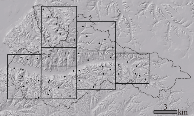
Figure 4 Zones and test areas (represented as points). The limits of the two studied basins are represented with a dashed line |
Table 4 Characteristics of the distributions of absolute error obtained for each interpolation method (i.e. square root of the square of the difference between real and interpolated values). Methods are ordered by ascending mean absolute error (MAE). Spline Reg and Spline Ten respectively identify the Regularized and Tension methods; w = weight parameter; P50 and P80 are the 50th and 80th percentiles; SD - standard deviation. All values are in metres. |
| Method | MAE | Min | Max | P50 | P80 | SD |
|---|---|---|---|---|---|---|
| Topo to Raster (contours) | 0.752 | 0.000 | 5.399 | 0.440 | 1.203 | 0.872 |
| Spline Reg w=0.01 | 0.767 | 0.000 | 5.001 | 0.463 | 1.176 | 0.889 |
| Spline Reg w=0.1 | 0.771 | 0.000 | 5.395 | 0.470 | 1.218 | 0.913 |
| Spline Reg w=0.001 | 0.810 | 0.000 | 5.338 | 0.493 | 1.239 | 0.904 |
| Spline Reg w=0.5 | 0.813 | 0.000 | 5.827 | 0.473 | 1.242 | 1.000 |
| Spline Reg w=0 | 0.834 | 0.000 | 5.456 | 0.526 | 1.288 | 0.912 |
| Spline Ten w=1 | 0.887 | 0.000 | 5.375 | 0.540 | 1.496 | 0.939 |
| Spline Ten w=4 | 0.954 | 0.000 | 5.354 | 0.587 | 1.654 | 0.976 |
| Spline Ten w=7 | 0.998 | 0.000 | 5.349 | 0.619 | 1.758 | 1.004 |
| Spline Ten w=10 | 1.034 | 0.000 | 5.350 | 0.639 | 1.828 | 1.028 |
| Linear | 1.214 | 0.000 | 6.908 | 0.815 | 1.962 | 1.239 |
| Topo to Raster (points) | 1.589 | 0.000 | 12.773 | 1.094 | 2.383 | 1.795 |
| Spline Ten w=0 | 3.463 | 0.001 | 72.642 | 1.084 | 3.494 | 7.500 |
Table 5 Characteristics of the distributions of absolute error obtained during parameter optimization. Methods are ordered by ascending mean absolute error (MAE).; w = weight parameter in the regularized (Reg) Spline method; R = roughness penalty in the Topo to Raster method; P50 and P80 are the 50th and 80th percentiles; SD - standard deviation. All values are in metres. |
| Method | Mean | Min | Max | P50 | P80 | SD |
|---|---|---|---|---|---|---|
| Spline Reg w=0.033 | 0.758 | 0.001 | 5.206 | 0.458 | 1.160 | 0.890 |
| Spline Reg w=0.055 | 0.762 | 0.001 | 5.291 | 0.468 | 1.191 | 0.896 |
| Spline Reg w=0.078 | 0.766 | 0.000 | 5.349 | 0.466 | 1.190 | 0.905 |
| Spline Reg w=0.008 | 0.771 | 0.000 | 5.042 | 0.463 | 1.171 | 0.890 |
| Spline Reg w=0.006 | 0.776 | 0.000 | 5.095 | 0.466 | 1.175 | 0.892 |
| Spline Reg w=0.003 | 0.791 | 0.000 | 5.210 | 0.480 | 1.191 | 0.897 |
| Topo to Raster R=0.4 | 0.825 | 0.000 | 5.499 | 0.496 | 1.318 | 0.922 |
| Topo to Raster R=0.3 | 0.871 | 0.000 | 4.920 | 0.547 | 1.442 | 0.923 |
| Topo to Raster R=0.2 | 0.938 | 0.000 | 5.585 | 0.618 | 1.519 | 0.980 |
| Topo to Raster R=0.1 | 0.987 | 0.000 | 5.634 | 0.664 | 1.599 | 1.007 |
| Topo to Raster R=0.5 | 1.020 | 0.000 | 5.716 | 0.701 | 1.635 | 1.029 |
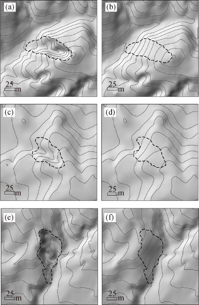
Figure 5 Three examples of surface reconstructions using the optimal interpolation method and parameterization (Topo to Raster with roughness penalty R = 0 and contours as input). (a), (c), (e) - original topography; (b), (d), (f) - reconstructed surfaces |
The authors have declared that no competing interests exist.
| 1 |
|
| 2 |
|
| 3 |
|
| 4 |
|
| 5 |
|
| 6 |
|
| 7 |
|
| 8 |
|
| 9 |
|
| 10 |
|
| 11 |
|
| 12 |
|
| 13 |
|
| 14 |
|
| 15 |
|
| 16 |
|
| 17 |
|
| 18 |
|
| 19 |
|
| 20 |
|
| 21 |
|
| 22 |
|
| 23 |
|
| 24 |
|
| 25 |
|
| 26 |
|
| 27 |
|
| 28 |
|
| 29 |
|
| 30 |
|
| 31 |
|
| 32 |
|
| 33 |
|
| 34 |
|
/
| 〈 |
|
〉 |