
Journal of Geographical Sciences >
Sequential city growth: Theory and evidence from the US
*Corresponding author: Sun Wei (1975-), Associate Professor, E-mail: sunw@igsnrr.ac.cn
Author: Sheng Kerong (1977-), Associate Professor, specialized in economic geography. E-mail: shengkerong@163.com
Received date: 2014-01-26
Accepted date: 2014-02-18
Online published: 2014-06-20
Supported by
National Natural Science Foundation of China, No.41230632.Key Project for the Strategic Science Plan in IGSNRR, CAS, No.2012ZD006
Copyright
City growth patterns are attracting more attention in urban geography studies. This paper examines how cities develop and grow in the upper tail of size distribution in a large-scale economy based on a theoretical model under new economic geography framework and the empirical evidence from the US. The results show that cities grow in a sequential pattern. Cities with the best economic conditions are the first to grow fastest until they reach a critical size, then their growth rates slow down and the smaller cities farther down in the urban hierarchy become the fastest-growing ones in sequence. This paper also reveals three related features of urban system. First, the city size distribution evolves from low-level balanced to primate and finally high-level balanced pattern in an inverted U-shaped path. Second, there exist persistent discontinuities, or gaps, between city size classes. Third, city size in the upper tail exhibits conditional convergence characteristics. This paper could not only contribute to enhancing the understanding of urbanization process and city size distribution dynamics, but also be widely used in making effective policies and scientific urban planning.
SHENG Kerong , SUN Wei , FAN Jie . Sequential city growth: Theory and evidence from the US[J]. Journal of Geographical Sciences, 2014 , 24(6) : 1161 -1174 . DOI: 10.1007/s11442-014-1145-8
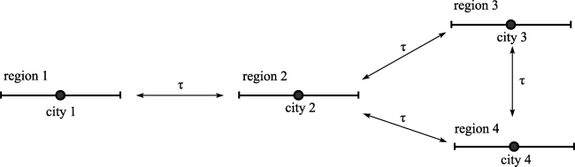
Figure 1 The spatial configuration of economic activities |
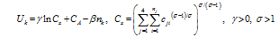
 and the rent subsidy per person is f nk/4. Thus, the living cost is g(d) +fd- f nk/4= f nk/4.) we will see in subsequent analysis, living cost is a major constraint for city size expansion.
Figure 2 The urban spatial structure |


 represents the quantity of a variety consumed in region k produced in region j, of which pjk represents the delivered price of a variety in region j imported from region k. For example, the price charged in region 4 for a variety produced in region 2 is p24=τp, and that charged in region 1 from region 3 is p31=2τp. Pk is the price index for the manufactured goods in region k, given by:


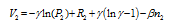
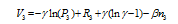

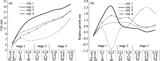
Figure 3 Numerical stimulations of city growth |
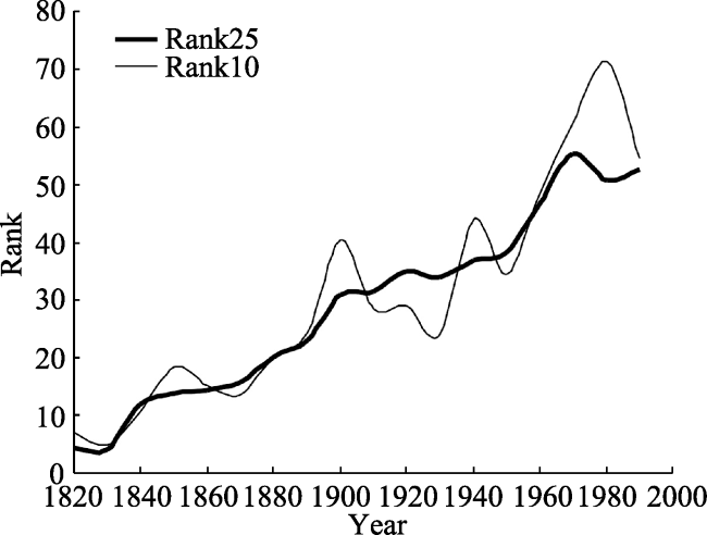
Figure 4 Evolution of Rank25 and Rank10 for US urban system, 1820-2000 |
Table 1 Regressions of Rank25 and Rank10 on time for US urban system, 1820-2000 |
| Rank25 | Rank10 | |||||
|---|---|---|---|---|---|---|
| (I) | (II) | (III) | (IV) | (V) | (VI) | |
| t | 2.873*** (0.206) | 2.076** (0.703) | 3.263*** (0.581) | -0.943 (1.721) | ||
| t2 | 0.143*** (0.012) | 0.042 (0.036) | 0.177*** (0.025) | 0.223** (0.087) | ||
| ln(number) | 1.212** (0.518) | 4.134*** (0.407) | 1.959** (0.807) | 0.822 (1.464) | 3.740*** (0.792) | 4.729** (1.977) |
| R2 | 0.969 | 0.956 | 0.97 | 0.830 | 0.887 | 0.884 |
| DW值 | 1.728 | 1.172 | 1.86 | 1.325 | 1.651 | 1.631 |
Note: Robust standard errors in the parentheses; ** and *** denote significance at 5% and 1% level, respectively. |
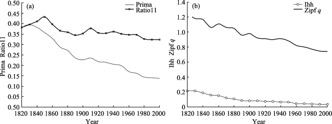
Figure 5 The evolution of Prima, Ratio11, Ihh and Zipf q for US urban system, 1820-2000 |
Table 2 Regressions of Prima, Ratio11, Ihh and Zipf q for US urban system, 1820-2000 |
| Prima | Ratio11 | IvIhh | Zipf q | |
|---|---|---|---|---|
| (VII) | (VIII) | (IX) | (X) | |
| t | -0.007** (0.003) | -0.004*** (0.001) | 2.157*** (0.312) | -0.016*** (0.004) |
| ln(number) | -0.065*** (0.019) | -5.702** (2.275) | -0.078** (0.032) | |
| cont | 0.547*** (0.049) | 0.403*** (0.007) | 16.262** (5.892) | 1.399*** (0.075) |
| R2 | 0.968 | 0.699 | 0.953 | 0.976 |
Note: Robust standard errors in the parentheses; ** and ***denote significance at 5% and 1% level, respectively. |
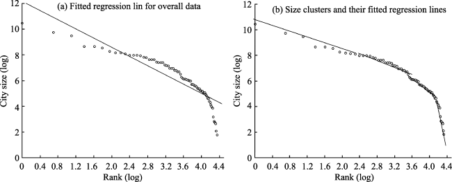
Figure 6 Hierarchical clusters in the US city size distribution in 1900 |
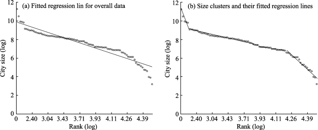
Figure 7 Hierarchical clusters in the US city size distribution in 1950 |

 of which
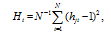
  and Sjt is the population size of city j.
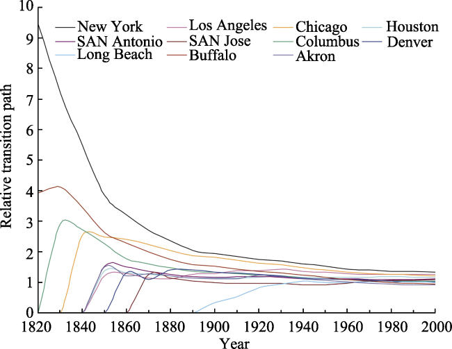
Figure 8 Relative transition paths for selected cities in the upper tail of the US urban system, 1820-2000 |
The authors have declared that no competing interests exist.
| 1 |
|
| 2 |
|
| 3 |
|
| 4 |
|
| 5 |
|
| 6 |
|
| 7 |
|
| 8 |
|
| 9 |
|
| 10 |
|
| 11 |
|
| 12 |
|
| 13 |
|
| 14 |
|
| 15 |
|
| 16 |
|
| 17 |
|
| 18 |
|
| 19 |
|
| 20 |
|
| 21 |
|
| 22 |
|
| 23 |
|
| 24 |
|
| 25 |
|
| 26 |
|
/
| 〈 |
|
〉 |
