Research Articles

An approach to spatially explicit reconstruction of historical forest in Northeast China

  • LI Shicheng , 1, 2 ,
  • HE Fanneng , *, 1 ,
  • ZHANG Xuezhen 1
Expand
  • 1. Key Laboratory of Land Surface Pattern and Simulation, Institute of Geographic Sciences and Natural Resources Research, CAS, Beijing 100101, China
  • 2. University of Chinese Academy of Sciences, Beijing 100049, China

*Corresponding author: He Fanneng, Professor, specialized in historical geography. E-mail:

Author: Li Shicheng, PhD Candidate, specialized in land use and land cover change. E-mail:

Received date: 2014-06-10

  Accepted date: 2014-07-02

  Online published: 2014-06-20

Supported by

China Global Change Research Program, No.2010CB950901.National Natural Science Foundation of China, No.41271227

Copyright

Journal of Geographical Sciences, All Rights Reserved

Abstract

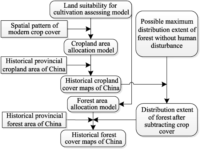
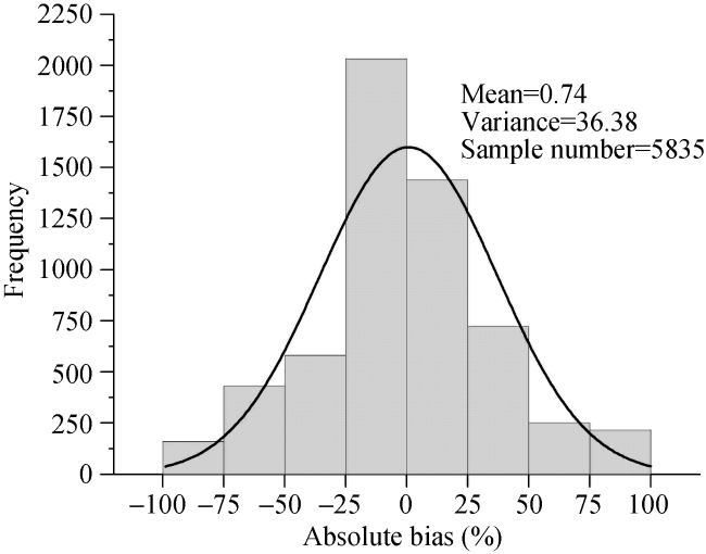
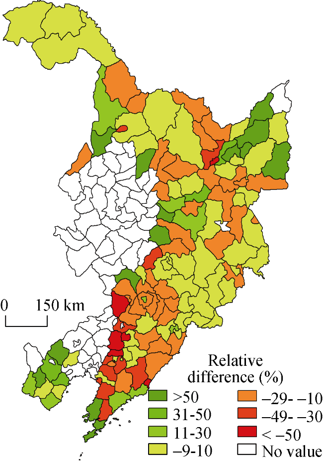
The spatially explicit reconstruction of historical land-cover datasets plays an important role in studying the climatic and ecological effects of land-use and land-cover change (LUCC). Using potential natural vegetation (PNV) and satellite-based land use data, we determined the possible maximum distribution extent of forest cover in the absence of human disturbance. Subsequently, topography and climate factors were selected to assess the suitability of land for cultivation. Finally, a historical forest area allocation model was devised on the basis of the suitability of land for cultivation. As a case study, we used the historical forest area allocation model to reconstruct forest cover for 1780 and 1940 in Northeast China with a 10-km resolution. To validate the model, we compared satellite-based forest cover data with our reconstruction for 2000. A one-sample t-test of absolute bias showed that the two-tailed significance was 0.12, larger than the significant level 0.05, suggesting that the model has strong ability to capture the spatial distribution of forests. In addition, we calculated the relative difference of our reconstruction at the county scale for 1780 in Northeast China. The number of counties whose relative difference ranged from -30% to 30% is 99, accounting for 74.44% of all counties. These findings demonstrated that the provincial forest area could be transformed into forest cover maps well using the model.

Cite this article

LI Shicheng , HE Fanneng , ZHANG Xuezhen . An approach to spatially explicit reconstruction of historical forest in Northeast China[J]. Journal of Geographical Sciences, 2014 , 24(6) : 1022 -1034 . DOI: 10.1007/s11442-014-1135-x

1 Introuduction

Human land use activities have substantially changed the land surface (Vitousek et al., 1997; Ellis et al., 2013), contributing to climate change, changes to the carbon and hydrological cycles, and a loss of biodiversity (Foley et al., 2005). Much attention has therefore been paid to studies on land-use and land-cover change (LUCC) and its effects (Ciais et al., 2011; Kaplan et al., 2011; Houghton et al., 2012). As one of the most important research fields of LUCC, the reconstruction of land cover spanning a long timescale is crucial in assessing the consequences of human land use activities (Ramankutty and Foley, 1999a), since the historical land cover datasets could serve as a basis for studies of the impact of historical LUCC on climate and calculations of carbon emissions over the last few centuries (Pongratz et al., 2010; He et al., 2014).
Since the 1990s, some international organizations or projects have devoted much attention to historical land use and land cover reconstruction, particularly in the past 300 years (Thompson, 2000; Miao et al., 2013; Yang et al., 2014). For instance, the Center for Sustainability and the Global Environment (SAGE) created a global cropland dataset for the period AD 1700-1992 with a resolution of 0.5° (Ramankutty and Foley, 1999b) and this dataset was updated in 2010 (Ramankutty and Foley, 2010). The History Database of the Global Environment (HYDE) was created by the Netherlands Environmental Assessment Agency via a novel method (Klein Goldewijk, 2001); the latest version, HYDE3.1, covers the past 12,000 years with a spatial resolution of 5′ (Klein Goldewijk et al., 2011). Based on historical population data and rational assumptions, Pongratz et al. (2008) expanded the reconstruction period of global cropland and pastureland cover to the past millennium. In addition, Kaplan et al. (2009) created a spatially explicit forest cover dataset of Europe over the past three millennia, using historical population data and maps of relative land suitability for crops and pastures. Later, these authors expanded the geographic scope to global and the entire period from 8000 years ago to AD 1850 using the same methods (Kaplan et al., 2011). By merging satellite imagery with census data, Leite et al. (2012) reconstructed a 5′ spatial resolution yearly dataset of land use from 1940 to 1995 for three different categories (cropland, natural pastureland, and planted pastureland) for Brazil. These reconstructions have all paid more attention to cropland and pastureland, whereas there are hardly any reconstructions of historical forest cover, particularly for China. Moreover, the deforestation datasets of Kaplan et al. (2009; 2011) were recreated based on the relationship between forest cover and population rather than using the essential historical records on forest area.
In terms of China, He et al. (2008) estimated the provincial forest area and forest coverage rate of China for 1700-1998 at 50-year intervals, based on historical records from the Qing Dynasty (AD 1616-1911) and modern inventories. Ye et al. (2009b) estimated the county-level forest cover in Northeast China over the past three centuries by cross-calibrating cropland area data from a number of historical documents, as well as using potential natural vegetation (PNV) data. These historical-document-based reconstructions provided data at the level of the political unit and thus could not be used directly in climatic or ecological models to study the effects of LUCC. Liu and Tian (2010) recreated forestland area changes in China from 1700 to 2005 according to satellite-based crop cover data and long term historical survey data at a resolution of 10 km. However, their assumption that the spatial relative weight of historical land use remained constant over the last 300 years is probably irrational (Houghton and Hackler, 2003).
Forests form a major part of the terrestrial ecosystem, and spatially explicit forest cover datasets spanning a long timescale are urgently needed to quantify the role that human beings played in the global carbon cycle. However, nowadays rational approaches to reconstructing the historical forest cover of China are scarce. Therefore, in this study, through determination of the possible maximum distribution extent of forest in the absence of human disturbance and assessment of the land suitability for cultivation, a model allocating the provincial forest area into 10- by 10-km grids was developed. As a case study, the model was used to reconstruct forest cover in Northeast China for 1780 and 1940.

2 Analysis overview

It has been reported that China was extensively covered by forest, with forest coverage of 49.6%-64% in the pre-agricultural period (Ling, 1983; Zhao, 1996; Fan and Dong, 2001). As society has developed and the population has increased over the past few centuries, deforestation has been widespread.
Some studies concerning the forest change history of China have indicated that deforestation was mainly caused by human land reclamation activities, particularly over the past few centuries (Ma et al., 1997; Fan and Dong, 2001). During the land reclamation process, land with good natural conditions, i.e., flat, low altitude, close to rivers, suitable sunshine and temperature, and easy to reach, will be cultivated first, followed by marginal lands with harsh natural environments further away from settlements (Wu, 1996; Wang, 2005; Han, 2012). In other words, land that is highly suited for cultivation will be cultivated and deforested first, followed by land that is less suitable for cultivation. Based on this analysis, we devised a methodology to reconstruct the historical forest cover of China in a spatially explicit way (Figure 1).
Figure 1 Reconstruction model for historical forest cover of China
First, we determined the possible maximum distribution extent of forest (MDEF) in the absence of human disturbance (Section 3.1). Then, we assessed the land suitability for cultivation (Section 3.2). Finally, combining the MEDF and the land suitability for cultivation for each province, we devised a provincial forest area allocation model based on the principle that the lands most suitable for cultivation would be deforested first (Section 3.3).

3 Reconstruction model

3.1 Possible maximum distribution extent of forest without human disturbance

PNV is widely used to study historical changes of land cover caused by human activities (Ramankutty and Foley, 1999b; Pongratz et al., 2008). The 5′ resolution global PNV map developed by Ramankutty and Foley (1999b; hereafter, RF99) is meant to be used only for continental-global scale applications, and some uncertainties might exist at the regional scale (Ramankutty and Foley, 2010; Zhang et al., 2011; Levavasseur et al., 2013). Because of the unavailability of a regional PNV map for China, the MDEF was determined to constrain the extent of forest allocation based on RF99 and satellite-based data.
It is possible that contemporary forest regions observed by satellite sensors were also forest regions in history, since human activities there are scarce. In terms of contemporary non-forest regions (e.g., traditional cultivated regions, built-up regions) observed by satellite sensors, it is likely that forest also existed in these regions in the past, including the North China Plain and the Sichuan Basin of China. As a result, we assumed that contemporary forest regions observed by satellite were also forest regions in history and that contemporary non-forest regions observed by satellite sensors were possible forest regions in history, but that their distribution does not exceed the forest regions reflected in the PNV map. In this study, PNV was used to replace the forest regions dominated by land use.
Based on these assumptions, we devised an algorithm to determine the possible MDEF in the absence of human disturbance (Figure 2). First, we overlaid several available satellite-based forest-cover maps of China and flagged all the grid cells with forest coverage greater than zero; all these flagged grid cells were classified as contemporary forest regions. Then, cultivated and built-up regions observed by satellite sensors in contemporary non-forest regions were replaced by RF99 to identify historical forest distribution regions in current land-use regions. Finally, contemporary forest regions and identified historical forest distribution regions in current land-use regions were combined, to obtain the MDEF. This may be taken as the possible distribution extent of forest that would exist at a given location if land use had never existed, which was in equilibrium with current climatic conditions.
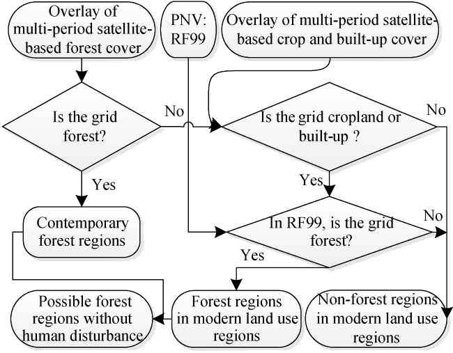
Figure 2 Flow chart to determine possible maximum distribution extent of forest in the absence of human disturbance

3.2 Land suitability for cultivation assessment model

As mentioned previously, historical deforestation was mainly caused by human agricultural activities in China (Ma et al., 1997; Fan and Dong, 2001). Moreover, land with high suitability for cultivation would be deforested first, followed by land with a harsh natural environment (Wang, 2005; Han, 2012). Therefore, the suitability of land for cultivation was assessed in this work to allocate the provincial forest area to grid cells.
3.2.1 Selecting factors affecting land suitability for cultivation
As one of the natural properties of land resources, the suitability of land for cultivation is jointly determined by topography, climate, river, and soil. Altitude, surface slope, and aspect are included in topography. Altitude will cause the vertical variation of hydrothermal conditions. Generally, with an increase in altitude, accumulated temperature no less than 10°C will decrease at a rate of 150-200 °C per 100 m, and the growing season will also be shortened (Department of Economic Geography in the Institute of Geography of the Chinese Academy of Sciences, 1980). Surface slope is closely related to soil erosion, land drainage, and irrigation. There is no soil erosion when the slope is below 3°. Soil erosion is common when the slope ranges from 3° to 15°, and serious soil erosion will occur on lands with a slope greater than 25° (Sun and Shi, 2003). That is to say, altitude and surface slope are closely related to land suitability for cultivation. In addition, different aspects will receive different amounts of sunshine, which contributes to different hydrothermal conditions. Nevertheless, the different hydrothermal conditions caused by aspect will not be reflected in the 10- by 10-km grid cell size. Aspect only affects the crop type and cropping system at the 10-km scale. In conclusion, altitude and surface slope were used to assess the land suitability for cultivation.
Climate is an index consisting of precipitation, temperature, and radiation. As the third biggest country in the world, China has various types of climate. If the combination of precipitation, temperature, and radiation is suitable for growing crops, then the land is suitable for cultivation; otherwise it is not (Smit and Cai, 1996). Thus, climate is an important factor affecting the suitability of land for cultivation.
In China, irrigation was advanced even in archaic periods, especially in the traditional cultivated regions of China (Wu, 1996), so the distance from rivers plays a minor role in determining land suitability for cultivation. At the 10-km scale, soil type mainly determines whether the land is suitable for cultivation, and its effects on reclamation are incorporated in the present cropland scope (Sun and Shi, 2003). In conclusion, three factors, i.e., altitude, surface slope, and potential maximum productivity of climate, were selected to model the land suitability for cultivation assessment.
3.2.2 Assessment of land suitability for cultivation
Based on the criteria derived from Sun and Shi (2003; Table 1), we reclassified and reassigned the altitude and slope value before normalization, as used by Lin et al. (2009) to quantify the impact of altitude and slope on cropland distribution.
The following equations were used in each province kn (n =1, 2, …, 25) to calculate the relationship between altitude, surface slope, climate, and land suitability for cultivation, respectively:
Table 1 Reclassification and reassignment of altitude and surface slope (Sun and Shi, 2003)
Altitude level (m) Reassigned value (m) Slope level (°) Reassigned value (°)
≤100 100 ≤2 2
100-250 250 2-6 6
250-500 500 6-15 15
500-750 750 15-25 25
750-1000 1000 >25 45
1000-1500 1500
1500-2000 2000
2000-3000 3000
>3000 4000
Combining these three normalized factors, we calculated the land suitability for cultivation assessment model as Equation (4), and the same weighting was assigned to each factor:
where δsuit(i) is the land suitability value for cultivation of grid i in province kn.
We can see that as altitude and slope increase, the land suitability for cultivation δsuit decreases, but that as climatic potential productivity value increases, the land suitability for cultivation δsuit increases too.

3.3 Devising historical forest area allocation model

Deforestation is closely related to land cultivation. Before we devised the historical forest area allocation model, we created a historical cropland area allocation model.
3.3.1 Cropland area allocation model
The provincial cropland area was allocated within the present cropland scope according to the spatial weighting of the cropland for each grid with a cell size of 10- by 10-km. As cropland was characterized by expansion in the past few centuries, almost all historical cropland was distributed within the present cropland scope. In this study, we used satellite-based cropland data for the early 1980s to denote the present cropland scope, as the cropland area reached a maximum in the early 1980s for the second half of the 20th century (Feng et al., 2005). By overlaying the 10- by 10-km grids on the 1-km satellite-based cropland dataset from Liu et al. (2005; 2014), we could determine whether there was cropland in the 10- by 10-km grid. As a result, we obtained a Boolean crop cover extent map φcrop(i) for the grid i in province kn. For φcrop(i), 1 indicates that there is cropland in this grid, and 0 indicates no cropland.
Using φcrop(i) and the land suitability for cultivation value δsuit(i), the cropland area of province kn in year t, area(kn, t), was fitted to a grid with a size of 10- by 10-km. The equations are as follows:
where β(i) is the spatial weight of cropland for grid i in province kn; and cropland(i, t) is the cropland area of grid i in year t.
3.3.2 Forest area allocation model
Next, based on the land suitability for cultivation assessment model and the MDEF, we devised a provincial forest area allocation model. The maximum value of forest area in each grid is 100 km2 (10 km × 10 km = 100 km2). Initially, the crop cover derived in Section 3.3.1 was subtracted from the MDEF (Equation (7)) to ensure that the cropland and forest area would not exceed 100 km2 in one grid.
where fremain(i, t) is the remaining forest area of grid i in year t after the subtraction of cropland area.
Within the remaining forest distribution extent, the provincial forest area of province kn in year t, farea(kn, t), was allocated to 10- by 10-km grids based on the reciprocal of the land suitability for cultivation value.
where fresult(i, t) is the forest area of grid i in year t.
It is important to note that some grids exist whose land suitability for cultivation value is high and perhaps the value of fresult(i, t) will be less than zero in these grids. In this situation, zero is assigned to fresult(i, t) of these grids. And the deforested area exceed zero in these grids will deforested in other grids of the same province whose fresult(i, t) values are greater than zero. The process was looped until each grid’s value of fresult(i, t) was greater than zero.

4 Case study and uncertainty analysis

4.1 Study area

As one of the major forest regions of China, Northeast China (including Liaoning, Jilin, and Heilongjiang) was selected as the case study area (Figure 3). Over the past few centuries, the forest coverage of Northeast China has changed dramatically. In particular, since the abolition of the ‘Prohibit Reclamation in Northeast China’ policy in 1860 by the Emperor Guangxu, farmers from Shandong, Shanxi, and Jing-Jin-Ji (including Beijing, Tianjin, and Hebei) migrated freely into Northeast China to deforest.
The territory and political units of the three provinces have changed over past centuries. To combine historical data with modern investigational data, the current territory and political units of the three provinces were used in this study.

4.2 Data sources

Forest area data were derived from Ye et al. (2009b). These county-level data are available for 1683, 1780, 1940, and 2000. These data were estimated based on historical documents, PNV, and driving force analysis, and reflected the actual forest area situation of Northeast China from 1683 to 2000. The data for 1780 and 1940 (Table 2) were selected and allocated into 10- by 10-km grid cells.
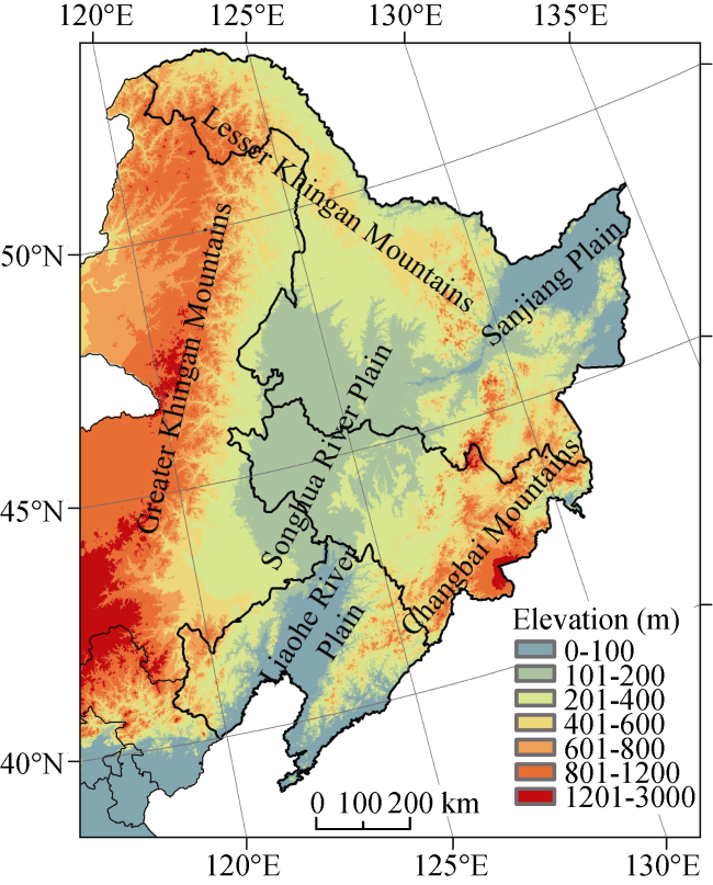
Figure 3 Location of the study area
In addition, the following data were also used: (1) cropland area data based on historical documents (Ye et al., 2009a); (2) satellite-based 1-km land-use data for the 1980s with an interpretation accuracy larger than 95% (Liu et al., 2005; 2014; available at http://www.geodata.cn); (3) PNV data (Ramankutty and Foley, 1999b); (4) the 1-km GTOPO30 dataset (http:// eros.usgs. gov/#/Find_Data/Products_and_Data_Available/Elevation_Products); (5) potential maximum productivity of climate data (http://www.geodata.cn). All these data were pre-processed to ensure consistent spatial resolution, 10- by 10-km, and the same geographic projection: the Lambert conformal conic projection.
Table 2 Forest area of Northeast China for 1780 and 1940 (km2)
Province 1780 1940
Liaoning 67946 12233
Jilin 118209 59863
Heilongjiang 282362 163650

4.3 Results and uncertainty analysis

4.3.1 Results
Figure 4 illustrates the forest cover of Northeast China for 1780 and 1940. In 1780, the distribution extents of forest were highly widespread and the forest coverage was large, which is consistent with records in historical documents such as The History and Geography of Northeast China (《朔方备乘》), The Brief History of Ningguta (《宁古塔纪略》) and The History Records of the Outside of Shanhai Pass (《柳边纪略》). The forest was mainly distributed in the Lesser Khingan Mountains, the Changbai Mountains, the Sanjiang Plains, and the western Liaoning Province. For 1940, the distribution extent of forest is much less than that for 1780. The forest hardly existed in the Sanjiang Plains and the western Liaoning Province, and the forest scope also shrank greatly in the Lesser Khingan Mountains and the Changbai Mountains. This was mainly caused by the abolition of the ‘Prohibit Reclamation in Northeast China’ policy in the second half of the 19th century.
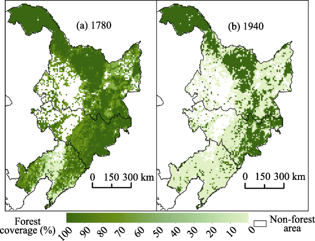
Figure 4 Forest cover of Northeast China for 1780 and 1940
4.3.2 Uncertainty analysis
Because of the absence of historical land cover maps, it is difficult to validate our reconstruction directly. In this study, by comparison with satellite-based data, we validated our reconstruction models; and by comparison with historical-record-based data at the county level, we analyzed the uncertainties of our reconstruction at the regional scale.
We reconstructed the forest cover for 2000 using our model, and provincial forest area data were aggregated from satellite-based forest cover data in 2000 to ensure that they are consistent with satellite-based data. Then we compared our reconstruction with satellite-based forest cover data for 2000; the comparison result is presented in Figure 5.
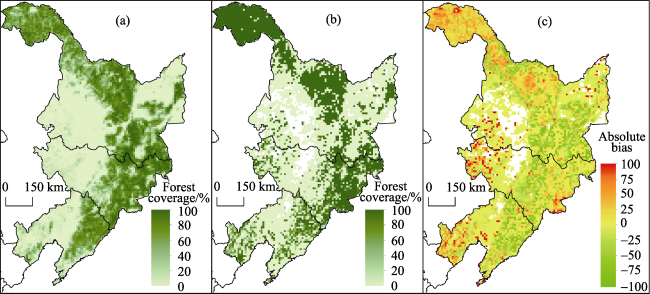
Figure 5 (a) Satellite-based forest cover in 2000; (b) Reconstructed forest cover in 2000; (c) Absolute bias of (a) and (b)
Generally, our reconstruction (Figure 5b) shows a similar spatial distribution of forest as the historical record-based data (Figure 5a). Both plots show that the forest is mainly distributed in the Lesser Khingan Mountain and the Changbai Mountain regions, and the differences for these regions mostly range from -25% to 25% (Figure 5c).
Figure 6 Distribution of absolute bias E(i)
In addition, the one-sample t-test of absolute bias (Figure 5c) was used to check whether there is a significant difference between the results. As shown in Figure 6, the absolute bias generally follows a normal distribution. Moreover, the one-sample t-test is a very robust statistical method, and the number of grids in this area is 5835, which is very large. Therefore, it is appropriate to validate our reconstruction models using the one- sample t-test method. The null hypothesis of the one-sample t-test is that there is no significant difference between our reconstruction and the satellite-based data. The test results are shown in Table 3. The t statistic is 1.55, and the two-tailed significance is 0.12, which is larger than the significance level of 0.05. Therefore, the null hypothesis cannot be refused and the bias is not statistically significant.
Table 3 One-sample t-test of absolute bias between satellite-based data and reconstruction results
Test mean = 0
T df Significance (2-tailed) Mean 95% confidence interval of the difference
Lower Upper
1.55 5834 0.12 0.74 -0.20 1.67
Figure 7 and Table 4 present comparison results between our reconstruction and the historical record-based data at the county level (Ye et al., 2009b). From Figure 7, we can see that the relative difference of our reconstruction at the county level is low overall. The difference value for the Lesser Khingan Mountain and the Changbai Mountain regions mostly ranges from -9% to 10% and a small portion ranges from -30% to -10%. The relative difference for the Sanjiang Plains and the hilly regions in the western Liaoning is mostly larger than 50%, whereas that of the hilly regions in the eastern Liaoning is mostly smaller than -50%.
Figure 7 Relative difference of our reconstruction in 1780 of Northeast China at the county scale
The number of counties whose relative difference ranges from -10% to 10% is 48, accounting for 36.09% of all counties (excluding missing data). A difference of -30% to -10% was found for 42 counties, and a difference of 10% to 30% for 9 counties, accounting for 31.58% and 6.77% of all counties, respectively. The number of counties whose relative difference is larger than 50% (>50% or <-50%) is 20, accounting for 15.04% of all counties (Table 4).
Table 4 Statistics of relative difference of our reconstruction in 1780 of Northeast China at the county scale
Relative difference (%) <-50 -50 to -30 -30 to -10 -10 to 10 10 to 30 30 to 50 >50 Missing data
Number of counties 6 10 42 48 9 4 14 51
Fraction of counties (%) 4.51 7.52 31.58 36.09 6.77 3.01 10.53

5 Conclusions and discussion

Combining satellite-based LUCC data and RF99, we determined the MDEF. Selecting and quantifying factors affecting land suitability for cultivation, we devised a land suitability for cultivation assessment model. Based on the principle that the land most suitable for cultivation will be deforested first, followed by marginal areas with low suitability for cultivation, a historical provincial forest area allocation model was created. In addition, the model was used to reconstruct the spatial pattern of forest cover in Northeast China for 1780 and 1940.
By comparing our reconstruction with satellite-based forest cover data for 2000, we found that the one-sample t-test of absolute bias showed that the two-tailed significance was 0.12, larger than the significance level 0.05, suggesting that the reconstruction method that we devised was rational. The relative difference at the county scale of our reconstruction for 1780 in Northeast China was calculated; the number of counties, whose relative difference ranges from -30% to 30%, is 99, accounting for 74.44% of all counties. This comparison indicated that the model could reflect the spatial distribution of forest well.
Although the comparison showed that our reconstruction had no significant difference from satellite-based forest-cover data, some uncertainties may exist in our reconstruction. From Figure 5, we can see that more forests were allocated into regions at relatively high altitudes in our reconstruction, including the north of Heilongjiang, the Lesser Khingan Mountains, the peak regions of Changbai Mountains, and the hilly regions of western Liaoning, while the distribution extents of our reconstruction are narrower than those of the satellite-based data in the transitional zones between the foothills and plains, such as the transitional zone between the east of Changbai Mountains and Sanjiang Plains. The relative difference of our reconstruction at the county scale also indicated that we allocated more forest area into regions with high altitude (Figure 7). It is possible that we only used land suitability for cultivation as a weighting to allocate provincial forest area without considering population, mining, transportation, and war factors, which might lead to the overweighting of topographical factors. Owing to the absence of historical population, economy data, and their complex relationship with forest cover, we omitted these factors in this study. Once they become available in future, incorporating them into our subsequent model might improve the accuracy of our reconstruction model.

The authors have declared that no competing interests exist.

1
Ciais P, Gervois S, Vuichard Net al., 2011. Effects of land use change and management on the European cropland carbon balance.Global Change Biology, 17(1): 320-338.

2
Department of Economic Geography in the Institute of Geography of Chinese Academy of Sciences, 1980. General Chinese Agricultural Geography. Beijing: Science Press, 1-454. (in Chinese)

3
Ellis E C, Kaplan J O, Fuller D Qet al., 2013. Used planet: A global history.Proceedings of the National Academy of Sciences of the United States of America, 110(20): 7978-7985.

4
Fan B M, Dong Y, 2001. A discussion on China’s ancient forest coverage.Journal of Beijing Forestry University, 23(4): 60-65. (in Chinese)

5
Feng Z M, Liu B Q, Yang Y Z, 2005. A study of the changing trend of Chinese cultivated land amount and data reconstructing: 1949-2003.Journal of Natural Resources, 20(1): 35-43. (in Chinese)

6
Foley J A, DeFries R, Asner G Pet al., 2005. Global consequences of land use.Science, 309(5734): 570-574.

7
Han M L, 2012. Historical Agricultural Geography of China. Beijing: Peking University Press, 13-47. (in Chinese)

8
He F, Vavrus S J, Kutzbach J Eet al., 2014. Simulating global and local surface temperature changes due to Holocene anthropogenic land cover change.Geophysical Research Letters, 41(2): 623-631.

9
He F N, Ge Q S, Dai J Het al., 2008. Forest change of China in recent 300 years.Journal of Geographical Sciences, 18(1): 59-72.

10
Houghton R A, Hackler J L, 2003. Sources and sinks of carbon from land-use change in China.Global Biogeochemical Cycles, 17(2): 1034.

11
Houghton R A, House J I, Pongratz Jet al., 2012. Carbon emissions from land use and land-cover change.Biogeosciences, 9(12): 5125-5142.

12
Kaplan J O, Krumhardt K M, Ellis E Cet al., 2011. Holocene carbon emissions as a result of anthropogenic land cover change.Holocene, 21(5): 775-791.

13
Kaplan J O, Krumhardt K M, Zimmermann N, 2009. The prehistoric and preindustrial deforestation of Europe.Quaternary Science Reviews, 28(27/28): 3016-3034.

14
Klein Goldewijk K, 2001. Estimating global land use change over the past 300 years: The HYDE Database.Global Biogeochemical Cycles, 15(2): 417-433.

15
Klein Goldewijk K, Beusen A, van Drecht Get al., 2011. The HYDE 3.1 spatially explicit database of human-induced global land-use change over the past 12,000 years.Global Ecology and Biogeography, 20(1): 73-86.

16
Leite C C, Costa M H, Soares-Filho B Set al., 2012. Historical land use change and associated carbon emissions in Brazil from 1940 to 1995. Global Biogeochemical Cycles, 26: GB2011.

17
Levavasseur G, Vrac M, Roche D Met al., 2013. An objective methodology for potential vegetation reconstruction constrained by climate.Global and Planetary Change, 104(2013): 7-22.

18
Lin S S, Zheng J Y, He F N, 2009. Gridding cropland data reconstruction over the agricultural region of China in 1820.Journal of Geographical Sciences, 19(1): 36-48.

19
Ling D X, 1983. Changes of forest resources in China.Agricultural History of China, (2): 26-36. (in Chinese)

20
Liu J Y, Kuang W H, Zhang Z Xet al., 2014. Spatiotemporal characteristics, patterns, and causes of land-use changes in China since the late 1980s.Journal of Geographical Sciences, 24(2): 195-210.

21
Liu J Y, Liu M L, Tian H Qet al., 2005. Spatial and temporal patterns of China's cropland during 1990-2000: An analysis based on Landsat TM data.Remote Sensing of Environment, 98(4): 442-456.

22
Liu M L, Tian H Q, 2010. China's land cover and land use change from 1700 to 2005: Estimations from high-resolution satellite data and historical archives. Global Biogeochemical Cycles, 24: GB3003.

23
Ma Z L, Song C S, Zhang Q H, 1997. The Change of China Forest. Vol. 45. Beijing: China Forestry Publishing House, 13-28. (in Chinese)

24
Miao L J, Zhu F, He Bet al., 2013. Synthesis of China’s land use in the past 300 years.Global and Planetary Change, 100: 224-233.

25
Pongratz J, Reick C, Raddatz Tet al., 2008. A reconstruction of global agricultural areas and land cover for the last millennium. Global Biogeochemical Cycles, 22(3): GB3018.

26
Pongratz J, Reick C H, Raddatz Tet al., 2010. Biogeophysical versus biogeochemical climate response to historical anthropogenic land cover change.Geophysical Research Letters, 37: L08702.

27
Ramankutty N, Foley J A, 1999a. Estimating historical changes in land cover: North American croplands from 1850 to 1992.Global Ecology and Biogeography, 8(5): 381-396.

28
Ramankutty N, Foley J A, 1999b. Estimating historical changes in global land cover: Croplands from 1700 to 1992.Global Biogeochemical Cycles, 13(4): 997-1027.

29
Ramankutty N, Foley J A, 2010. ISLSCP II historical croplands cover, 1700-1992

(Data set). In: Hall F G, Collatz G, Meeson Bet al. eds. ISLSCP Initiative II Collection. [http://daac.ornl.gov/] from Oak Ridge National Laboratory Distributed Active Archive Center, Oak Ridge, TN, USA.

30
Smit B, Cai Y L, 1996. Climate change and agriculture in China.Global Environmental Change, 6(3): 205-214.

31
Sun H, Shi Y L, 2003. China Agricultural Land Use. Nanjing: Jiangsu Science and Technology Publishing House, 3-84. (in Chinese)

32
Thompson R S, 2000. BIOME 300: Understanding the impacts of human activities on land cover over the past 300 years.IGBP Newsletter, 43: 2-3.

33
Vitousek P M, Mooney H A, Lubchenco Jet al., 1997. Human domination of Earth's ecosystems.Science, 277(5325): 494-499.

34
Wang Y H, 2005. Chinese historical land use. In: Wang G, Wang J, Wang P eds. Proceedings of Wang Yuhu. Beijing: China Agricultural Press. (in Chinese)

35
Wu C H, 1996. Chinese Agricultural History. Beijing: Police-Education Press, 1-1295. (in Chinese)

36
Yang Y Y, Zhang S W, Yang J Cet al., 2014. A review of historical reconstruction methods of land use/land cover.Journal of Geographical Sciences, 24(4): 746-766.

37
Ye Y, Fang X Q, Ren Y Yet al., 2009a. Cropland cover change in Northeast China during the past 300 years. Science in China Series D: Earth Sciences, 52(8): 1172-1182.

38
Ye Y, Fang X Q, Zhang X Zet al., 2009b. Coverage changes of forestland and grassland in northeastern China during the past 300 years.Journal of Beijing Forestry University, 31(5): 137-144. (in Chinese)

39
Zhang X Z, Wang W C, Fang X Qet al., 2011. Vegetation of Northeast China during the late seventeenth to early twentieth century as revealed by historical documents.Regional Environmental Change, 11(4): 869-882.

40
Zhao G, 1996. China Environmental Change. Beijing: China Environmental Science Press, 1-10. (in Chinese)

Outlines

/