
Journal of Geographical Sciences >
Evolving a core-periphery pattern of manufacturing industries across Chinese provinces
 is the share of industry k in region i, popi is the share of the whole country’s population living in region i, and mani is the share of the total manufacturing located in region i. The new economic geography believes that the historic economy is important to industry growth; hence, pathi is added in the model to control for the effect of path dependence, presented by the scale of same industry lagged by 5 years. In an open economy, foreign investment and international trade also have effects on industrial distribution, hence foreign market access fdmi is applied in the model to measure geographical advantage on foreign economic activity for one region, calculated by the inverse distance from a region to the coast; α, β, σ, τ, γj are regression coefficients, and θj and δj are critical levels. When estimating the equation, we need to derive estimates of the three key parameters for each interaction variable, that is, of θj, δj and γj. We also derive estimates for the impact of the two scale variables and the other controlling variables, that is, of α, β, σ, and τ. In the discussion of our results, we concentrate on γj which measures the sensitivity of all industries to variations in regional characteristics. Returning to the example of centrality, if the core-periphery dimension is an important determinant of industrial location, then we should obtain a high value of γj. If it equals θj, there is no preference by the industry to the region; if it is greater than θj, the industry preferring the core region tends to locate there, and if it is smaller than θj, the industry preferring the periphery regions tends to locate there. Correspondingly, δj measures certain characteristics of the industry, taking scale economy as an example. If it equals δj, the industry has no preference to any region; if it is smaller than δj, the industry tends to locate in core regions, and, the industry tends to locate in the periphery if it is greater than δj. If regional economic gradient determines the change of distribution disparity of industries with different eigenvalues for the scale economy, a high γj is expected, as well as other industrial characteristics. If γj is greater than 0, the industry with a high eigenvalue tends to locate in the corresponding area, and vice versa.
Author: Mao Qiliang, PhD, specialized in regional economics and industrial location. E-mail: more1987@163.com
Received date: 2014-01-15
Accepted date: 2014-02-16
Online published: 2014-05-20
Supported by
National Science and Technology Infrastructure Program of China, No.2007FY110300
Copyright
This paper, concerning uneven development in China, empirically analyzes the core-periphery gradient of manufacturing industries across provinces (autonomous regions, municipalities), and assesses the extent to which these provinces have changed in recent years. Since China’s reform and opening-up, the spatial structure of the economy has presented a significant core-periphery pattern, the core evidently skewing towards east-coastal areas. With the deepening of market reforms and expansion of globalization, industrial location is gradually in line with the development advantages of provinces. The core provinces specialize in those industries characterized by strong forward and backward linkages, as well as a high consumption ratio, a high degree of increasing returns to scale, and labor or human-capital intensity. However, it is the opposite with regard to peripheral provinces, in addition, energy intensive industries are gradually concentrating in these areas. To a certain degree, the comparative advantage theory and new economic geography identify the underlying forces that determine the spatial distribution of manufacturing industries in China. This paper indicates that the industrialization of regions along different gradients becomes unsynchronized will be a long-term trend. Within a certain period, regions are bound to develop industrial sectors in line with their respective characteristics and development stage. A core-periphery pattern of industries also indicates that industrial development differentials across regions arise because of not only the uneven distribution of industries but also the inconsistent evolving trends of industrial structure for each province.
MAO Qiliang , WANG Fei , LI Jun , DONG Suocheng . Evolving a core-periphery pattern of manufacturing industries across Chinese provinces[J]. Journal of Geographical Sciences, 2014 , 24(5) : 924 -942 . DOI: 10.1007/s11442-014-1129-8
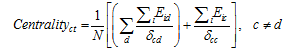
Table 1 Indicators of industrial characteristic |
| Industrial characteristic | Measurement | |
|---|---|---|
| j = 1 | Intermediate input ratio | Intermediate inputs, % of output |
| j = 2 | Ultimate consumption ratio | Domestic consumption, % of total sale |
| j = 3 | Scale economy | Employment per enterprise |
| j = 4 | Labor intensity | Percentage of labor wage in output, % of output |
| j = 5 | Higher skills intensity | Share of higher educated workers in workforce |
| j = 6 | Energy intensity | Energy consumption per output, ton standard coal |
| j = 7 | Tax rate | Percentage of tax in output, % of output |
| j = 8 | State-owned enterprise raito | Percentage of state-owned enterprise in total enterprise, % of total enterprise |
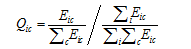
 is scale of industry i in region c,
  is scale of all industries in province c,
  is scale of industry i in all provinces, and
  is scale of all industries in all provinces.
 is the share of industry k in region i, popi is the share of the whole country’s population living in region i, and mani is the share of the total manufacturing located in region i. The new economic geography believes that the historic economy is important to industry growth; hence, pathi is added in the model to control for the effect of path dependence, presented by the scale of same industry lagged by 5 years. In an open economy, foreign investment and international trade also have effects on industrial distribution, hence foreign market access fdmi is applied in the model to measure geographical advantage on foreign economic activity for one region, calculated by the inverse distance from a region to the coast; α, β, σ, τ, γj are regression coefficients, and θj and δj are critical levels. When estimating the equation, we need to derive estimates of the three key parameters for each interaction variable, that is, of θj, δj and γj. We also derive estimates for the impact of the two scale variables and the other controlling variables, that is, of α, β, σ, and τ. In the discussion of our results, we concentrate on γj which measures the sensitivity of all industries to variations in regional characteristics. Returning to the example of centrality, if the core-periphery dimension is an important determinant of industrial location, then we should obtain a high value of γj. If it equals θj, there is no preference by the industry to the region; if it is greater than θj, the industry preferring the core region tends to locate there, and if it is smaller than θj, the industry preferring the periphery regions tends to locate there. Correspondingly, δj measures certain characteristics of the industry, taking scale economy as an example. If it equals δj, the industry has no preference to any region; if it is smaller than δj, the industry tends to locate in core regions, and, the industry tends to locate in the periphery if it is greater than δj. If regional economic gradient determines the change of distribution disparity of industries with different eigenvalues for the scale economy, a high γj is expected, as well as other industrial characteristics. If γj is greater than 0, the industry with a high eigenvalue tends to locate in the corresponding area, and vice versa.
 dividing the estimation of
  by γj. Similarly, industrial characteristic δj can be estimated. If the model is correct, the estimations of θj and δj are positive. If the estimation of γj appears in contradiction to
  then the revised model is as follows:
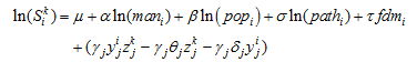
Table 2 Definition of independent variables |
| Regional characteristic ( | Industrial characteristic ( | Hypothesis | |
|---|---|---|---|
| j = 1 | Centrality (Centrality) | Intermediate input ratio (Input) | Hypothesis 1 |
| j = 2 | Centrality (Centrality) | Ultimate consumption ratio (Dmnd) | Hypothesis 2 |
| j = 3 | Centrality (Centrality) | Scale economy (Scale) | Hypothesis 3 |
| j = 4 | Labor endowment (L-endmnt) | Labor intensity (L-inten) | Hypothesis 4 |
| j = 5 | High skills- endowment (H-endmnt) | Higher skills intensity (H-inten) | Hypothesis 5 |
| j = 6 | Energy endowment (Eng-endmnt) | Energy intensity (Eng-inten) | Hypothesis 5 |
| j = 7 | Local protection (Local) | Tax rate (Tax) | Hypothesis 6 |
| j = 8 | Local protection (Local) | State-owned enterprise raito (State) | Hypothesis 6 |
Note: Letters in parentheses refer to regional and industrial characteristics. |
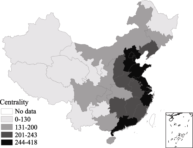
Figure 1 Centrality of GDP in the Provinces of China in 2008 |
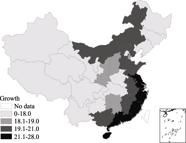
Figure 2 Variation of centrality of GDP in the provinces of China (1980-2008) |
Table 3 Correlation coefficients between location quotient and centrality index (1980-2008) |
| Sector | 1980 | 1985 | 1995 | 2004 | 2008 |
|---|---|---|---|---|---|
| Food processing | - | - | -0.4105** | -0.2229* | -0.3899** |
| Food production | -0.5044*** | -0.5248*** | -0.0590 | -0.1254 | -0.2046 |
| Beverage production | -0.2515 | -0.3488* | -0.2516 | -0.2970 | -0.2676 |
| Tabaco processing | -0.1824 | -0.2025 | -0.2215 | -0.1815 | -0.1810 |
| Feed manufacturing | 0.4954*** | 0.0718 | - | - | - |
| Textile industry | 0.2534 | 0.2205 | -0.0122 | 0.0159 | 0.0007 |
| Garments & other fiber products | - | - | 0.4604** | 0.3243* | 0.2247 |
| Leather, furs, down & related products | -0.1927 | -0.1982 | -0.0908 | 0.0447 | -0.0144 |
| Timber processing, bamboo, cane, palm fiber & straw products | -0.1036 | -0.1291 | -0.1991 | -0.1769 | -0.2915* |
| Furniture manufacturing | -0.3285** | -0.2417 | -0.1485 | 0.2593 | 0.2409 |
| Papermaking & paper products | -0.1241 | -0.1557 | -0.2946 | -0.0999 | -0.0863 |
| Printing & record pressing | -0.2045 | -0.1197 | -0.2138 | -0.0184 | -0.0246 |
| Stationery, educational & sports goods | 0.8618*** | 0.7963*** | 0.4633*** | 0.4412** | 0.3442* |
| Petroleum processing | -0.0587 | -0.1353 | - | - | - |
| Coking products, & gas production & supply | 0.4626** | 0.4010** | - | - | - |
| Petroleum processing, Coking products, & gas production & supply | - | - | -0.0575 | -0.1457 | -0.1552 |
| Raw chemical materials & chemical products | 0.1798 | 0.2416 | -0.0781 | -0.1218 | -0.1950 |
| Medical & pharmaceutical products | 0.1947 | 0.0521 | -0.0628 | -0.2211 | -0.2216 |
| Chemical fibers | 0.7643*** | 0.7979*** | 0.3251* | 0.0504 | 0.0064 |
| Rubber products | 0.0232 | 0.0796 | -0.0312 | 0.0664 | 0.0776 |
| Plastic products | 0.1082 | 0.1829 | 0.0462 | 0.2367 | 0.2562 |
| Nonmetal mineral products | -0.5341*** | -0.5941*** | -0.4634*** | -0.2413* | -0.3005* |
| Smelting & pressing of ferrous metals | 0.1792 | 0.1601 | 0.1648 | -0.0363 | -0.0167 |
| Smelting & pressing of nonferrous metals | -0.0692 | -0.0783 | -0.2389 | -0.2733 | -0.2877 |
| Metal products | 0.3268* | 0.4091** | 0.3639** | 0.5611*** | 0.5404*** |
| Machinery manufacturing | 0.0873 | 0.0730 | - | - | - |
| Machinery & equipment manufacturing | - | - | 0.2073 | 0.4077** | 0.4740*** |
| Special equipment manufacturing | - | - | 0.0235 | 0.1615 | 0.2795 |
| Transportation equipment manufacturing | -0.1849 | -0.1822 | 0.1512 | 0.0274 | 0.1411 |
| Electric equipment & machinery | 0.3733** | 0.2818 | 0.3335* | 0.3674** | 0.3403* |
| Electronic & telecommunications | 0.5434*** | 0.3652** | 0.4736*** | 0.6469*** | 0.7024*** |
| Instruments, meters, cultural & official machinery | 0.2826 | 0.2894 | 0.5641*** | 0.4860*** | 0.5477*** |
Note: * = significant at 5% level; ** = significant at 10%. To simply page allocation, standard errors haven’t been reported. “-” refers no data. |
Table 4 Results of the least square estimation |
| 1985 | 1995 | 2004 | 2008 | |
|---|---|---|---|---|
| Interactions | ||||
| Centrality×Input | 0.1434 (0.0881) | 0.1024*** (0.0243) | 0.0446*** (0.0118) | 0.0269*** (0.0076) |
| Centrality×Dmnd | 0.0292 (0.0268) | 0.0309*** (0.0071) | 0.0160*** (0.0034) | 0.0101*** (0.0022) |
| Centrality×Scale | 0.0201*** (0.0074) | -0.0021 (0.0030) | 0.0010* (0.0015) | 0.0019* (0.0028) |
| L-endmnt×L-inten | -0.0001 (0.0034) | 0.0001* (0.0000) | -0.0001 (0.0000) | 0.0001 (0.0000) |
| Hc-endmnt×Hc-inten | -0.0016 (0.0049) | -0.0006 (0.0008) | -0.0007* (0.0004) | -0.0002 (0.0002) |
| Eng-endmnt×Eng-inten | 0.0717 (0.0500) | 0.0778*** (0.0301) | 0.0849*** (0.0264) | 0.0582*** (0.0187) |
| Other variables | ||||
| Manu | 0.8834*** (0.1208) | 0.7545*** (0.0957) | 0.6721*** (0.1247) | 0.5921*** (0.1325) |
| Pop | 0.1633 (0.1596) | 0.3467** (0.1258) | 0.4683*** (0.1539) | 0.5977*** (0.1670) |
| Fdm | -0.0550 (0.1084) | 0.0030* (0.0691) | 0.1558* (0.0898) | 0.1879** (0.0933) |
| Path | 0.8939*** (0.0127) | 0.9083*** (0.0207) | 1.0111*** (0.0285) | 0.9258*** (0.0177) |
| Local×Tax | 22.6602 (15.6260) | 19.7197 (10.7284) | 2.4767 (2.7029) | 1.4283 (1.3357) |
| Local×State | 56.1146* (36.8005) | 35.7379** (26.6363) | 27.3633* (16.6759) | 2.7619 (3.3154) |
| Adjusted R-squared | 0.8466 | 0.8614 | 0.8840 | 0.8295 |
| S.E. | 0. 653 | 0. 721 | 0. 701 | 0. 692 |
| Number of obs | 765 | 826 | 866 | 872 |
Note: Standard errors reported in brackets; * = significant at 5% level; ** = significant at 10%. S.E. refers standard errors. All regressions are overall significant according to the standard F-test. |
Table 5 Results of estimation by two stages least square |
| 1985 | 1995 | 2004 | 2008 | |
|---|---|---|---|---|
| Interactions | ||||
| Centrality×Input | -0.1499 (0.3638) | 0.1727** (0.0448) | 0.0483*** (0.0133) | 0.0277*** (0.0077) |
| Centrality×Dmnd | -0.0013 (0.0403) | 0.0337** (0.0078) | 0.0155*** (0.0034) | 0.0102*** (0.0021) |
| Centrality×Scale | 0.0314*** (0.0098) | 0.0097 (0.0076) | 0.0146** (0.0056) | 0.0071** (0.0038) |
| L-endmnt×L-inten | -0.0034 (0.0061) | -0.0001 (0.0001) | -0.0002** (0.0001) | -0.0001** (0.00003) |
| Hc-endmnt×Hc-inten | 0.0015 (0.0055) | 0.0009 (0.0010) | 0.0011* (0.0007) | 0.0051** (0.0002) |
| Eng-endmnt×Eng-inten | 0.0850 (0.0522) | 0.0787** (0.0318) | 0.0880*** (0.0292) | 0.0536*** (0.0200) |
| Other variables | ||||
| Man | 0.8982*** (0.1201) | 0.7701*** (0.0973) | 0.6702*** (0.1231) | 0.6284*** (0.1298) |
| Pop | 0.1492 (0.1586) | 0.3331*** (0.1276) | 0.4692*** (0.1519) | 0.5818*** (0.1649) |
| Fdm | -0.0560 (0.1076) | 0.0027** (0.0700) | 0.156*** (0.0887) | 0.1881** (0.0411) |
| Path | 0.8989*** (0.0134) | 0.9183*** (0.0231) | 1.0435*** (0.0334) | 0.9239*** (0.0176) |
| Local×Tax | -7.8106 (26.3684) | 9.0357 (6.7800) | 0.3379 (2.9996) | 1.4541 (1.3498) |
| Local×State | 43.0539** (44.0992) | 37.4653** (28.7800) | 17.7382* (9.3935) | 2.6360* (3.4418) |
| Adjusted R-squared | 0.8411 | 0.8573 | 0.8278 | 0.8264 |
| S.E. | 0. 639 | 0. 711 | 0. 693 | 0. 671 |
| Number of obs | 765 | 826 | 866 | 872 |
Note: Standard errors reported in brackets; * = significant at 5% level; ** = significant at 10%. S.E. refers to standard errors. All regressions are overall significant according to the standard F-test. |
The authors have declared that no competing interests exist.
| 1 |
|
| 2 |
|
| 3 |
|
| 4 |
|
| 5 |
|
| 6 |
|
| 7 |
|
| 8 |
|
| 9 |
|
| 10 |
|
| 11 |
|
| 12 |
|
| 13 |
|
| 14 |
|
| 15 |
|
| 16 |
|
| 17 |
|
| 18 |
|
| 19 |
|
| 20 |
|
| 21 |
|
| 22 |
|
| 23 |
|
| 24 |
|
| 25 |
|
| 26 |
|
| 27 |
|
| 28 |
|
| 29 |
|
| 30 |
Vernon, 1966. International investment and international trade in the product cycle.The Quarterly Journal of Economics, 2(80): 190-207.
|
| 31 |
|
| 32 |
|
| 33 |
|
| 34 |
|
| 35 |
|
| 36 |
|
/
| 〈 |
|
〉 |