Research Articles

Water resource utilization efficiency and spatial spillover effects in China

  • SUN Caizhi , 1 ,
  • ZHAO Liangshi 1 ,
  • ZOU Wei 2 ,
  • ZHENG Defeng 1
Expand
  • 1. Urban and Environment School of Liaoning Normal University, Dalian 116029, Liaoning, China
  • 2. Foreign Language School of Liaoning Normal University, Dalian 116029, Liaoning, China

Author: Sun Caizhi (1970-), Professor, specialized in water resources evaluation and management. E-mail:

Received date: 2014-03-30

  Accepted date: 2014-04-22

  Online published: 2014-05-20

Supported by

National Social Science Foundation of China, No.11BJY063.Program for New Century Excellent Talents in University, No.NECT-13-0844

Copyright

Journal of Geographical Sciences, All Rights Reserved

Abstract

Based on provincial panel data of water footprint and grey water footprint, and with the help of data envelopment analysis model considering and without considering the undesirable output, this paper estimates the water resources utilization efficiency in China from 1997 to 2011. The spatial weighting matrix based on economy-spatial distance function is established to discuss spatial autocorrelation of water resources utilization efficiency. With the help of absolute β-convergence model, this paper concludes that there exists β-convergence in the water resources utilization efficiency. Under the conditions of considering and without considering the undesirable output, it takes about 52.6 and 5.6 years respectively to achieve the extent of half of convergence. By mean of the spatial Durbin econometric model, this paper studies spatial spillover effects of the provincial water resources utilization efficiency in China. The results are as follows. 1) With considering and without considering the undesirable output, there is significant spatial correlation in provincial water resource efficiency in China. 2) Under the two cases, the spatial autoregressive coefficients (ρ) are 0.278 and 0.507 respectively, at 1% significance level. There exist the spatial spillover effects of provincial water resources utilization efficiency. 3) With considering the undesirable output, these factors of the education funds, the transportation infrastructure, and the industrial and agricultural water consumption proportion have positive impacts. These factors of foreign direct investment, the industry value-added water consumption per ten thousand yuan, per capita water consumption, and the total precipitation have negative impacts. 4) Without considering the undesirable output, the factor of GDP per laborer has a greater positive significant influence on the water resources utilization efficiency. However the facts of industry value-added water consumption in ten thousand yuan and the transportation infrastructure have no significant influence. 5) Regardless of undesirable output of water resources utilization efficiency, the assessment of the present real water resources utilization in China will be distorted and policy-making will be misled. The water efficiency measure considering environmental factors (such as gray water footprint) is more reasonable.

Cite this article

SUN Caizhi , ZHAO Liangshi , ZOU Wei , ZHENG Defeng . Water resource utilization efficiency and spatial spillover effects in China[J]. Journal of Geographical Sciences, 2014 , 24(5) : 771 -788 . DOI: 10.1007/s11442-014-1119-x

1 Introduction

China is currently facing two critical issues in terms of water resource management: shortage of water resources and deterioration in the quality of aquatic ecosystems. Spatial distribution of water resources in the country is extremely uneven. The per capita water availability is about 2200 m3, which is only a quarter of the global average. Inefficiency of water use further adds to the problem of water shortage in the country. According to China Water Resources Bulletin, 80.7 billion t of water was discarded in 2011, as compared to 58.4 billion t in 1997. This suggests an increase in the quantity of discarded water, by 38.2%, during these years. Efficient utilization of water resources, thus, becomes imperative for China to maintain a sustainable water supply.
Several models have been developed in the past to evaluate production efficiencies. Data Envelopment Analysis (DEA), proposed by Charnes and Cooper (1978), is one of the most commonly used models. It was used to assess the relative water resource utilization efficiency through an evaluation of efficiencies of the decision-making units (DMUs) (Sun et al., 2009). The undesirable output radial direction DEA model was used to measure the water resources utilization relative environmental technology efficiency of 31 provinces (autonomous regions and municipalities) in China, from 1997 to 2010 (Sun et al., 2013). In an earlier attempt, an index of a water adjustment target ratio (WATR) was established from the production frontier constructed through DEA - including water as an input - and water efficiency of the selected regions was obtained from a total-factor framework, with both residential and productive water use (Hu et al., 2006). However, the traditional DEA model did not take the problem of input and output relaxation into consideration. The Slack-Based Measure (SBM) was introduced by Tone to deal with inputs and outputs individually (2001, 2003). It was used to measure the total factor energy efficiency of 30 provinces, from 1999 to 2010, based on the undesirable output (Fan et al., 2013). Based on the same model, the agricultural eco-efficiency of 30 provinces in China was measured from 1998 to 2009 (Pan et al., 2013). This paper aims to overcome the shortcoming of the traditional DEA models - by utilizing the SBM model based on the undesirable output - to measure the water resource utilization efficiency of 31 provinces in China from 1997 to 2011.
Spatial spillover effects are widely studied and can be drawn from both regional development and economics literature (Anselin, 2003, Audretsch, 2003). The phenomenon can imply a variety of meanings, such as knowledge spillover (Fischer, 2006), industry spillover (Audretsch et al., 2004), growth spillover (Arora et al., 2005) and a variety of fields have benefitted by employing the model. For instance, the relationship between total factor productivity and infrastructure and its spatial spillover effect was tested by using spatial Durbin economic model (Zhang et al., 2012). Using the spatial Durbin model, based on the Cobb-Douglas (C-D) production function and on the panel data from provinces, an empirical study on the knowledge spillovers effects was implemented in China (Liu et al., 2010). The regional spillovers of the transport infrastructure stock in Chinese regions were also estimated using the spatial Durbin Model (Yu et al., 2013). The broader effects - including direct and spatial spillover effects - of transportation infrastructure on the agricultural output across 44 states in the United States were estimated from 1981 to 2004 (Tong et al., 2013). Using the method of MEDD, the evolution of spatial distribution dynamics of provincial economic growth was explored, from the aspects of shape and mobility, in China from 1978 to 2004 (Li et al., 2007). Based on the spatial spillover effect of the real estate prices, the house exchange price data of Guangzhou city in 2005 was used to explore the border effect of administrative districts within the city by applying extended Hedonic model and semi-variogram function (Hong et al., 2011). Using a panel dataset of two-digit manufacturing industries in Beijing during the period 1999-2004, a study found that geographically agglomerated industries with strong intra-industrial linkages attract much foreign investment (He et al., 2006).
Spatial spillover models, as explained above, are widely employed across various fields of study. However, there are rare studies on the spatial spillover effects of water resources utilization efficiency, and there are even less studies taking environmental factors into consideration. Water resource utilization efficiency refers to the economic, social, and ecological benefits brought by water consumption in a unit. The spatial spillovers effects in this regard refer to the diffusion of beneficial effects of enhanced water resource utilization efficiency in one region to the other adjacent regions. Such spillovers can act as counter-balance measures for the uneven distribution of water resources and lead to natural resources endowment in China. Therefore, it is important to not only demonstrate these effects, but also to quantify the spillovers.
Based on the above understanding, this paper aims to measures the water resources utilization efficiency of 31 provinces in China, from 1997 to 2011, by employing SBM model based on the undesirable output. It uses water footprint, labor and capital as inputs; GDP as the desirable output; and grey water footprint as the undesirable output. Spatial weights matrix based on economy-spatial distance function is established to discuss the spatial autocorrelation of water resources utilization efficiency. It also uses the Spatial Durbin econometric model to study the spatial spillovers of the provincial water resources utilization efficiency in China.

2 Methodology

First, the paper estimates the water resources utilization efficiency in China by applying the SBM model and taking the undesirable output into consideration. It, thereby, aims to get rid of the inefficiency factor caused by the relaxation problem in the conventional radial DEA model (Charnes et al., 1978). Second, the paper uses Moran’s I index to test the spatial autocorrelation of water resource utilization efficiency at the provincial scale. Third, absolute β-convergence model is utilized to verify the convergence of water resource utilization efficiencies in various provinces. Last, the water resource utilization efficiency spatial spillover effects are tested by spatial Durbin econometric model.

2.1 SBM with undesirable outputs

The paper builds the following constants return to scale model based on the relaxation and non-radial undesirable output SBM model (Tone, 2001, 2003):
where the objective function ρ is the water resources utilization efficiency. There are K×T DMUs and three factors associated with each DMU: inputs, good outputs, and undesirable outputs, as represented by three vectors and respectively. The input and output value of the first k×t DMU at t period is represented by vector . The vectors 
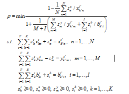
and denote input and output slack and the weight of K×T DMUs at t period respectively. The objective function ρ strictly decreases with respect to and the objective value satisfies . The first k’ DMU is efficient in the presence of undesirable outputs, if and only if ρ=1. While it is inefficient, i.e., ρ<1, it can be improved and made efficient by deleting the excesses in inputs and undesirable outputs and augmenting the shortfalls in desirable outputs.
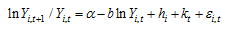
2.2 Absolute β-convergence model

While studying the neoclassical growth convergence, Barro and Sala-i-Martin (1992, 1996) constructed and applied the absolute β-convergence model. Absolute β-convergence with regard to our study implies that the regions with low water resources utilization efficiencies tend to grow faster than the ones with high efficiencies. Based on which, this paper sets up the following panel data econometric model of water utilization efficiency:
where Yi,t is the first i province’s water resource utilization efficiency at t period, hi is the fixed effect that reflects the difference among various provinces, kt is the fixed effect at different periods that mainly controls the factor of water resource utilization efficiency with change of periods, εi,t is the random disturbance term that remains unaffected by region as well as period. If b>0, the water resource utilization efficiency leads to absolute β-convergence, else it leads to divergence. The convergence speed is determined by the coefficient β.

2.3 Spatial Durbin econometric model

Spatial econometric writings tend to start from a particular theory or model and focus on the problems of estimation specification and testing when spatial effects are present. Spatial effects are the essential reason for the existence of a separate field of spatial econometrics (Anselin, 1988). Spatial econometricians are mainly interested in modeling the spatially autoregressive process in either the dependent variable or the error term. The former is known as the spatial lag model, whereas the latter refers to the spatial error model (Elhorst, 2010). However, the methodological limitations of both the spatial lag and spatial error models have not been explicitly addressed in the previous research. The spatial Durbin econometric model (Anselin, 1988) has been proven to outperform the spatial lag and spatial error models and address the aforementioned limitations. Under the spatial Durbin analytic framework, no restriction is imposed on the magnitude of the spatial effects, and both global and local effects are produced (Lesage et al., 2009). The spatial Durbin econometric model includes a spatial lag of the dependent variable as well as the explanatory variable, and a spatial lag of the explanatory variable. In a spatial context, externalities (both positive and negative) arising from neighborhood characteristics often have direct sensory impacts. In order to test the spatial spillover effects of water resource utilization efficiency in China, the spatial panel data Durbin econometric model in this paper can be written in the following way:
where Y, W, X, WX and ε denote the water resource utilization efficiency, the spatial weight matrix, the influencing factors of water resource utilization efficiency, and the explanatory variable of the influencing factors, respectively. In models containing spatial lags of the explanatory or dependent variables, interpretation of the parameters becomes richer and more complicated. LeSage and Pace (2009) provided some explanations about the parameters of spatial Durbin econometric model in the form of partial derivative matrix and proposed the definitions of average total impacts, average direct impacts and average indirect impacts. Taking these into account, equation (3) can be rewritten as:
On both side with time and denoted by:
where 
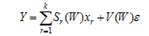
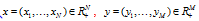
By expanding equation (5), we obtain the following:
The average total impacts, direct impacts and indirect impacts can be inferred from equation (6) as:
The average total impact is the average of all derivatives of yi with respect to xjr for any i and j. The average direct impact is the average of all own derivatives. The average of all derivatives (average total impact) less than the average own derivative (average direct impact) equals the average cross derivative (average indirect impact). The view expressed in equation (9) relates to how changes in a single observation j influence all observations (LeSage et al., 2009).

2.4 Spatial weight matrix

Our research on spatial dependence and spatial autocorrelation measurement of the water resource utilization efficiency in China is based on the assumption of adjacency relations between different regions. The original measures for spatial dependence were based on the notion of binary contiguity between spatial units. If two spatial units have a common border of non-zero length, they are considered contiguous and a value of 1 is assigned. The adjacency relation 0-1 ignores the effects derived from the actual geographic distance between two regions. The spatial adjacency relations based on distance function (Sun et al., 2013; Zhao et al., 2013), however, consider that the effect between two closer regions is larger, and vice versa. Spatial weight matrix elements based on distance function are defined as follows:
where dij is the distance between the center of gravity of the region i and region j. The weight matrix is symmetric and this assumption may be convenient from a measurement and modeling point of view. However, asymmetric spatial distance between two regions seems plausible and should be accommodated in applied modeling (Parent et al., 2008). Due to different levels of economic development in various regions, the economic relationships between them also vary. Incorporating the relative levels of economic activities for each region can be accomplished by modifying the proximity index from region i to j as below:
where GDPi/GDPj measures the output gap between regions i and j. Thus, the asymmetric effects between the technological distances Wij and Wji are more pronounced when the economic activity gap between regions i and j increases. The spatial weight matrix in this paper is row-standardized since the sum of the elements in each row is equal to 1.

3 Empirical results

3.1 Water resources utilization efficiency measurement

Based on provincial panel data of water footprint and grey water footprint, and with the help of data envelopment analysis model considering and without considering the undesirable output, next this paper estimates the water resources utilization efficiency in China from 1997 to 2011.
3.1.1 Index selection and data processing
The data of input and output water resource in China from 1997 to 2011 (not including Taiwan, Hong Kong, Macao) has been taken from China Statistical Yearbook (1998-2012), China Water Resources Bulletin (1997-2011), China Environment Yearbook (1998-2012) and the provincial statistical yearbook data. The missing data during particular periods in some parts has been filled by the adjacent areas’ approximation or fitting forecast values. Specific indicators are shown as follows:
(1) Water footprint:
This paper complements and revises the water footprint data found previously in literature (Sun et al., 2013, Zhao et al., 2013). We supplement the data of the water pollution footprint by taking the chemical oxygen demand (COD) and the ammonia nitrogen pollution footprint parameters into account; fill the missing ecological water consumption data for 1997-2002; and update the water footprint data until 2011. Water footprint reflects the direct and indirect water consumption. The goal of assessing water footprints is to quantify total and actual water consumption at a specific time and place and to assess the sustainability of the water consumption. Based on the water footprint assessment methodologies and research achievements of the predecessors [3, 20, 21, and 23-27], our paper presents the following equation for water footprint calculation:
where WF, WFcs, WFip, WFwp, and WFde denote the total water footprint, the urban and rural residents’ consumption of livestock products water footprint, the industrial products water footprint, the grey water footprint, and the life and ecological water footprint, respectively.
As shown in Figure 1, the average water footprint among provinces and cities in China from 1997 to 2011 differs greatly. The proportion of grey water footprint and livestock products is presumably different. The water footprints are relatively lower in Beijing, Tianjin, Shanghai, Hainan, Shanxi, Gansu, Qinghai, and Ningxia; and higher in Hebei, Jiangsu, Shandong, Guangdong, and Sichuan. This shows that the spatial distribution of the water footprint is not only related to the geographical space, but also to the degree of economic development and water resources endowment. As an indicator of water resource input, the water footprint reflects the real amount of the water resources consumed in the production of consumer products and services (Hoekstra, 2003).
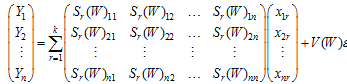
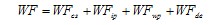
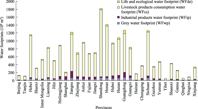
Figure 1 The composition of the water footprints in China
(2) Fresh water: The water sum of agricultural, industrial, life and ecological consumption.
(3) Labor force: The employee index measures the amount of labor for actual production processes.
(4) Fixed-asset investment: The fixed-asset investment as capital input is at 1990 for the base period.
(5) GDP: Gross domestic product (GDP) as the expected output is at 1990 for the base period.
(6) Grey water footprint: Considered by this paper as an undesirable output, it refers to the quantity of water required to dilute the pollutants, associated with the production of goods and services, in order to achieve the agreed water quality standard.
3.1.2 Water resources utilization efficiency measurement based on environmental regulation
Table 1 shows the water resources utilization efficiencies measured by considering the undesirable output SBM model, based on the panel data from 31 provinces and cities in China from 1997 to 2011. It also compares these efficiency values with the ones measured without considering the undesirable output.
Table 1 The l water resource utilization efficiency in various provinces of China from 1997 to 2011
Regions 1997 2001 2004 2008 2011 Average value
Beijing 0.134/0.196 0.210/0.316 0.287/0.383 0.587/0.539 1.000/0.759 0.414/0.423
Tianjin 0.115/0.165 0.182/0.284 0.257/0.398 0.487/0.639 0.885/1.000 0.344/0.476
Hebei 0.103/0.146 0.145/0.216 0.193/0.296 0.317/0.455 0.511/0.608 0.235/0.330
Shanxi 0.064/0.116 0.095/0.171 0.130/0.247 0.208/0.369 0.287/0.494 0.150/0.272
Inner Mongolia 0.050/0.080 0.076/0.117 0.114/0.186 0.227/0.367 0.356/0.534 0.152/0.240
Liaoning 0.111/0.190 0.163/0.295 0.217/0.390 0.352/0.606 0.581/0.877 0.265/0.449
Jilin 0.058/0.112 0.087/0.168 0.113/0.227 0.194/0.376 0.290/0.492 0.138/0.263
Heilongjiang 0.069/0.111 0.099/0.159 0.131/0.215 0.199/0.314 0.272/0.407 0.149/0.235
Shanghai 0.176/0.271 0.298/0.433 0.427/0.549 0.714/0.832 1.000/1.000 0.498/0.605
Jiangsu 0.164/0.206 0.258/0.319 0.369/0.430 0.646/0.665 1.000/1.000 0.457/0.497
Zhejiang 0.142/0.202 0.215/0.296 0.306/0.404 0.531/0.589 0.777/0.840 0.381/0.446
Anhui 0.069/0.100 0.099/0.141 0.129/0.181 0.205/0.266 0.293/0.358 0.153/0.202
Fujian 0.094/0.167 0.141/0.231 0.184/0.296 0.301/0.444 0.428/0.574 0.221/0.332
Jiangxi 0.045/0.073 0.067/0.105 0.087/0.142 0.135/0.211 0.192/0.278 0.102/0.157
Shandong 0.136/0.218 0.207/0.324 0.306/0.475 0.597/0.768 1.000/1.000 0.413/0.539
Henan 0.079/0.112 0.105/0.159 0.140/0.221 0.239/0.350 0.352/0.481 0.173/0.256
Hubei 0.087/0.126 0.129/0.186 0.163/0.243 0.264/0.365 0.386/0.468 0.197/0.268
Hunan 0.066/0.088 0.093/0.126 0.117/0.162 0.192/0.256 0.291/0.371 0.142/0.190
Guangdong 0.183/0.237 0.278/0.351 0.413/0.484 0.699/0.714 1.000/1.000 0.492/0.537
Guangxi 0.053/0.076 0.073/0.105 0.099/0.139 0.157/0.220 0.238/0.316 0.118/0.163
Hainan 0.045/0.071 0.059/0.098 0.072/0.123 0.105/0.179 0.149/0.251 0.082/0.139
Chongqing 0.063/0.125 0.092/0.176 0.121/0.229 0.198/0.348 0.344/0.593 0.152/0.273
Sichuan 0.093/0.143 0.133/0.203 0.179/0.272 0.295/0.420 0.490/0.635 0.221/0.315
Guizhou 0.030/0.054 0.042/0.072 0.053/0.091 0.084/0.138 0.135/0.233 0.064/0.107
Yunnan 0.054/0.081 0.071/0.106 0.088/0.135 0.130/0.190 0.181/0.270 0.101/0.149
Tibet 0.025/0.031 0.037/0.044 0.049/0.059 0.068/0.079 0.087/0.106 0.052/0.062
Shaanxi 0.048/0.090 0.074/0.141 0.100/0.196 0.168/0.319 0.241/0.458 0.120/0.227
Gansu 0.040/0.061 0.057/0.087 0.073/0.114 0.110/0.172 0.140/0.231 0.081/0.128
Qinghai 0.032/0.043 0.046/0.061 0.063/0.079 0.093/0.120 0.133/0.167 0.069/0.089
Ningxia 0.028/0.031 0.037/0.044 0.047/0.060 0.067/0.094 0.086/0.125 0.051/0.068
Xinjiang 0.055/0.065 0.210/0.089 0.089/0.113 0.126/0.160 0.156/0.201 0.097/0.123
In the case where undesirable output is considered, the water resources utilization efficiencies in all the provinces improve significantly between 1997 and 2011. However, there are huge differences between the provincial efficiencies for each period and the spatial distribution is also uneven. As can be seen, the utilization efficiencies in all provinces and cities improves gradually between 1997 and 2004 - from a minimum 0.025 for Tibet, in 1997, to a maximum 0.427 for Shanghai, in 2004. However, the values improve quickly between 2004 and 2011, with Beijing, Shanghai, Jiangsu, Shandong, and Guangdong reaching the water resources utilization efficiency 1 in 2011. In general, the efficiencies vary greatly among the different provinces and periods, with the arithmetic means of the efficiencies ranging from a minimum 0.051 to a maximum 0.498, between 1997 and 2011.
The results indicate that fluctuations in the water resources utilization efficiencies, in the case where undesirable output is not considered, is quite similar to where it is considered. The values improve by considerable margins on an annual basis. However, the overall efficiencies are higher where undesirable output is not considered. Another notable finding here is that there are interprovincial differences in efficiencies in both the cases. The measurements for Beijing, Tianjin, Shanghai, Jiangsu, Guangdong and other places in every period is high, while Shanxi, Tibet, Yunnan, Guizhou and other places reflect lower values. This indicates that there is an implicit connection between the water resources utilization efficiency and economic geographical spatial distribution in China.
3.1.3 Spatial autocorrelation test
Table 2 shows the global autocorrelation index value (Anselin, 1988) of the water resources utilization efficiency in China, from 1997 to 2011, for both the scenarios where undesirable output is considered and not considered. The values indicate existence of spatial agglomera- tion phenomenon at a significant level of 1%. This means that the spatial distribution of the water efficiencies in the country is not completely random, but demonstrates spatial agglomeration phenomenon between similar value regions, i.e. the higher value regions are clustered together. Thus, the econometric aspect of geographical spatial distribution cannot be ignored while studying the water resources utilization efficiencies in China. In addition, the two properties that can be considered in the context of spatial econometric analysis are spatial dependence and spatial heterogeneity.
Table 2 The Moran’s I of water utilization efficiency in China
Year Consider the undesirable output Year Without considering the undesirable output
Moran’s I z-Statistic P-value Moran’s I z-Statistic P-value
1997 0.0647 2.8350 0.0023 1997 0.0686 2.9467 0.0016
1998 0.0647 2.8355 0.0023 1998 0.0713 3.0254 0.0012
1999 0.0660 2.8740 0.0020 1999 0.0719 3.0426 0.0012
2000 0.0663 2.8831 0.0020 2000 0.0735 3.0902 0.0010
2001 0.0677 2.9211 0.0017 2001 0.0752 3.1393 0.0008
2002 0.0637 2.8075 0.0025 2002 0.0730 3.0746 0.0011
2003 0.0632 2.7931 0.0026 2003 0.0768 3.1855 0.0007
2004 0.0616 2.7451 0.0030 2004 0.0771 3.1934 0.0007
2005 0.0660 2.8745 0.0020 2005 0.0819 3.3312 0.0004
2006 0.0636 2.8047 0.0025 2006 0.0788 3.2415 0.0006
2007 0.0650 2.8429 0.0022 2007 0.0800 3.2777 0.0005
2008 0.0655 2.8586 0.0021 2008 0.0807 3.2969 0.0005
2009 0.0674 2.9134 0.0018 2009 0.0802 3.2815 0.0005
2010 0.0623 2.7669 0.0028 2010 0.0740 3.1034 0.0010
2011 0.0725 3.0606 0.0011 2011 0.0659 2.8702 0.0021
The next step is using local Moran’s index to find out whether local agglomeration phenomenon exists in terms of water resources utilization efficiencies in China. Figure 2 shows the LISA cluster map of the water resources utilization efficiency in China, for both cases - where undesirable output is considered and not considered. The H-H areas mainly concentrate in the eastern coastal regions and include areas such as Beijing, Tianjin, Hebei, Liaoning, Shandong, Shanghai, Jiangsu, Zhejiang, and Fujian. These exhibit a significant amount of the agglomeration phenomenon and form the water resources utilization high value efficiency areas. The L-L areas mainly concentrate in the western and central regions. These are away from the open economically developed coastal areas, and also exhibit the agglomeration phenomenon significantly. The L-H and H-L areas are located between H-H and L-L areas and do not manifest agglomeration phenomenon significantly.
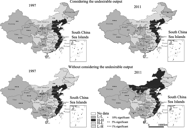
Figure 2 LISA map of water utilization efficiency in China

3.2 The spillover effects measurement

If the various Chinese provinces show a trend of concentration distribution from 1997 to 2011, then how do efficiencies on a provincial scale evolve and whether there is a possibility of convergence? Are there significant spatial spillover effects? How do different factors influence the water resources utilization efficiencies? These questions are further explored in the following sections, with reference to the regional economic development and policies on the water resources utilization.
3.2.1 The convergence test
Table 3 shows the absolutely β-convergence of the water resources utilization efficiency, measured with the help of equation (2). The convergence speed of water resources utilization efficiency for the two cases - where undesirable output is considered and not considered - is 0.013 and 0.115 respectively. This indicates that absolute β-convergence does exist and a 0.5 convergence speed can be attained in 52.6 and 2.6 years under the two scenarios respectively. As expected, the convergence speed is quite quick when undesirable output is not considered, which implies that various provinces in China could attain the same level of efficiencies in a short time span. While on the other hand, the convergence speed is slower when the undesirable output is considered. Therefore, it can be said that the assessment of current water resource utilization in China will produce distorted results if the undesirable output is not taken into consideration.
Table 3 Model regression results
Regression
result
Considering the undesirable output Regression
result
Without considering the undesirable output
Regression
coefficient
t-Statistic Regression
coefficient
t-Statistic
α 0.083** 2.125 α -0.074* -1.740
b 0.013 -0.691 b 0.109*** -4.131
Convergence rate β 0.013 Convergence rate β 0.115
R2 0.552 R2 0.424
Likelihood ratio 905.059 Likelihood ratio 913.031

Note: *** refers to 1% significant level; ** to 5% significant level; * to 10% significant level.

3.2.2 The regression results of spatial Durbin econometric model
As demonstrated with the help of spatial correlation analysis earlier, our findings indicate that an area’s water resource utilization efficiency is not only related to the economic development, but also to the water resource utilization efficiencies of the other adjoining areas. This autocorrelation, called spatial dependence, leads to spatial spillover effects. The phenomenon can help reduce the unevenness in the water resources utilization efficiencies across various provinces, thereby improving the overall water sustainability in China. Therefore, we now attempt to quantify the spatial effects related to the water resources utilization efficiency in the country, with the help of spatial Durbin econometric model. The data for the study has been obtained from China Statistical Yearbook (1998-2012) and China Water Resources Bulletin (1997-2011).
We utilize Hausman test (Baltagi, 2005) for the spatial Durbin econometric model and adopt only fixed effects and reject the random effects. Table 4 displays the results. The spatial autoregressive coefficients (ρ) are at 1% significance level for both the cases - where undesirable output is considered and not considered - which establishes that spatial spillover effects exist with regard to the water resources utilization efficiency in China. However, the spatial autoregressive coefficient (ρ) is 0.507 where undesirable output is not considered, and is 0.278 where undesirable output is considered.
Table 4 Model regression results
Variable Considering the
undesirable output
Variable Without considering the undesirable output
Regression
coefficient
t-Statistic Regression
coefficient
t-Statistic
Foreign direct investment (108 yuan) 0.017* 1.684 Foreign direct investment (108 yuan) 0.003 0.632
GDP per laborer (108 yuan) 0.449*** 9.011 GDP per laborer (108 yuan) 0.685*** 34.565
Transportation infrastructure (km) -0.021 -1.053 Transportation infrastructure (km) -0.021*** -2.661
Per capita water consumption (m3) -0.156*** -3.504 Per capita water consumption (m3) -0.178*** -10.005
Per ten thousand yuan industry value-added water consumption (m3) -0.045** -1.974 Per ten thousand yuan industry value-added water consumption (m3) -0.044*** -4.790
Per acre farmland irrigation water consumption (m3) 0.154*** 4.359 Per acre farmland irrigation water consumption (m3) 0.013 0.955
Education funds (104 yuan) -0.140*** -5.063 Education funds (104 yuan) -0.001 -0.003
Industrial water consumption proportion (%) -0.007 -0.256 Industrial water consumption proportion (%) 0.024*** 2.199
Agricultural water consumption proportion (%) -0.181*** -7.496 Agricultural water consumption proportion (%) -0.089*** -9.247
Marketization degree (%) 0.225*** 4.291 Marketization degree (%) 0.060*** 2.855
Total precipitation (108 m) -0.038** -2.148 Total precipitation (108 m) 0.002 0.219
Lag foreign direct investment (108 yuan) -0.359*** -6.304 Lag foreign direct investment (108 yuan) -0.069*** -3.066
Lag GDP per laborer (108 yuan) -0.269 -1.548 Lag GDP per laborer (108 yuan) -0.266*** -2.886
Lag transportation infrastructure (km) 0.247*** 4.013 Lag transportation infrastructure (km) 0.030 1.222
Lag per capita water consumption (m3) -0.223 -1.639 Lag per capita water consumption (m3) -0.102* -1.695
Lag per ten thousand yuan industry value-added water consumption (m3) -0.027 -0.543 Lag per ten thousand yuan industry value-added water consumption (m3) 0.046** 2.346
Lag per acre farmland irrigation water consumption (m3) 0.238 1.442 Lag per acre farmland irrigation water consumption (m3) 0.179*** 2.669
Lag education funds (104 yuan) 0.517*** 10.979 Lag education funds (104 yuan) 0.103*** 5.353
Lag industrial water consumption proportion (%) 0.524*** 7.102 Lag industrial water consumption proportion (%) 0.171*** 5.563
Lag agricultural water Lag consumption proportion (%) 0.641*** 8.041 Lag agricultural water Lag consumption proportion (%) 0.213*** 6.701
Lag marketization degree (%) -0.059 -0.410 Lag marketization degree (%) 0.020 0.354
Lag total precipitation (108 m) -0.214*** -2.932 Lag total precipitation (108 m) -0.116*** -3.903
ρ 0.278*** 3.198 ρ 0.507*** 7.492
R2 0.994 R2 0.998
Likelihood ratio 651.753 Likelihood ratio 1076.924

Note: *** refers to 1% significant level; ** to 5% significant level; * to 10% significant level.

In the case where we consider the undesirable output, the factors that significantly affect the water resources utilization efficiency are - foreign direct investment, transportation infrastructure, GDP per laborer, per capita water consumption, per ten thousand yuan industry value-added water consumption, per acre farmland irrigation water consumption, education funds, industrial water consumption proportion, agricultural water consumption proportion, marketization degree, and total precipitation. In the case where undesirable output is not considered, the factors that significantly affect the water resources utilization efficiency are - foreign direct investment, GDP per laborer, transportation infrastructure, per capita water consumption, per ten thousand yuan industry value-added water consumption, per acre farmland irrigation water consumption, education funds, industrial water consumption proportion, water consumption proportion, marketization degree, and total precipitation.
The regression model results are very good in terms of R2 and likelihood ratio. However, spatial Durbin econometric model regression coefficient does not directly reflect the impact of independent variables on dependent variables. It reflects spatial effects when total effects, direct effects, and indirect effects are taken into consideration (Table 5). The following discussion examines the effects of different factors on the water resources utilization efficiencies in terms of these effects.
Table 5 Total effect, direct effect and indirect effect of explanative variables
Considering the undesirable output Without considering the undesirable output
Total effects Regression
coefficient
t-Statistic Total effects Regression
coefficient
t-Statistic
Foreign direct investment (108 yuan) -0.475*** -4.786 Foreign direct investment (108 yuan) -0.138** -2.678
GDP per laborer (108 yuan) 0.243 1.042 GDP per laborer (108 yuan) 0.848*** 6.277
Transportation infrastructure (km) 0.312*** 3.289 Transportation infrastructure (km) 0.018 0.349
Per capita water consumption (m3) -0.518** -2.646 Per capita water consumption (m3) -0.571*** -4.713
Per ten thousand yuan industry value-added water consumption (m3) -0.104* -1.708 Per ten thousand yuan industry value-added water consumption (m3) 0.005 0.148
Per acre farmland irrigation water consumption (m3) 0.541** 2.251 Per acre farmland irrigation water consumption (m3) 0.391*** 2.746
Education funds (104 yuan) 0.525*** 6.006 Education funds (104 yuan) 0.212*** 4.483
Industrial water consumption proportion (%) 0.717*** 6.389 Industrial water consumption proportion (%) 0.400*** 5.899
Agricultural water consumption proportion (%) 0.641*** 4.442 Agricultural water consumption proportion (%) 0.258*** 3.472
Marketization degree (%) 0.225 1.179 Marketization degree (%) 0.165 1.461
Total precipitation (108 m) -0.349*** -3.068 Total precipitation (108 m) -0.234*** -3.506
Direct effects Regression
coefficient
t-Statistic Direct effects Regression
coefficient
t-Statistic
Foreign direct investment (108 yuan) 0.012 1.178 Foreign direct investment (108 yuan) -0.001 -0.033
GDP per laborer (108 yuan) 0.449*** 9.07 GDP per laborer (108 yuan) 0.688*** 34.042
Transportation infrastructure (km) -0.018 -0.908 Transportation infrastructure (km) -0.021** -2.519
Per capita water consumption (m3) -0.159*** -3.674 Per capita water consumption (m3) -0.185*** -9.806
Per ten thousand yuan industry value-added water consumption (m3) -0.046* -2.018 Per ten thousand yuan industry value-added water consumption (m3) -0.043*** -4.716
Per acre farmland irrigation water consumption (m3) 0.157*** 4.382 Per acre farmland irrigation water consumption (m3) 0.020 1.368
Education funds (104 yuan) -0.133*** -4.628 Education funds (104 yuan) 0.004 0.360
Industrial water consumption proportion (%) -0.001 -0.001 Industrial water consumption proportion (%) 0.031** 2.704
Agricultural water consumption proportion (%) -0.173*** -6.906 Agricultural water consumption proportion (%) -0.082*** -8.797
Marketization degree (%) 0.225*** 4.42 Marketization degree (%) 0.061*** 2.913
Total precipitation (108 m) -0.041** -2.253 Total precipitation (108 m) -0.003 -0.413
Indirect effects Regression
coefficient
t-Statistic Indirect effects Regression
coefficient
t-Statistic
Foreign direct investment (108 yuan) -0.487*** -5.103 Foreign direct investment (108 yuan) -0.138*** -2.795
GDP per laborer (108 yuan) -0.205 -0.898 GDP per laborer (108 yuan) 0.160 1.218
Transportation infrastructure (km) 0.33*** 3.491 Transportation infrastructure (km) 0.038 0.776
Total effects Regression
coefficient
t-Statistic Total effects Regression
coefficient
t-Statistic
Per capita water consumption (m3) -0.359* -1.925 Per capita water consumption (m3) -0.386*** -3.379
Per ten thousand yuan industry value-added water consumption (m3) -0.058 -0.885 Per ten thousand yuan industry value-added water consumption (m3) 0.048 1.287
Per acre farmland irrigation water consumption (m3) 0.385 1.654 Per acre farmland irrigation water consumption (m3) 0.372** 2.714
Education funds (104 yuan) 0.658*** 8.17 Education funds (104 yuan) 0.208*** 4.821
Industrial water consumption proportion (%) 0.717*** 6.759 Industrial water consumption proportion (%) 0.369*** 5.760
Agricultural water consumption proportion (%) 0.814*** 5.918 Agricultural water consumption proportion (%) 0.340*** 4.791
Marketization degree (%) -0.001 -0.005 Marketization degree (%) 0.103 0.929
Total precipitation (108 m) -0.308*** -2.851 Total precipitation (108 m) -0.231*** -3.625

Note: *** refers to 1% significant level; ** to 5% significant level; * to 10% significant level.

In terms of total effects, when undesirable output is considered, the factors such as education funds, transportation infrastructure, and proportion of industrial and agricultural water have positive impacts; whereas, foreign direct investment, and per ten thousand yuan industry value-added water consumption have negative impacts. However, without considering the undesirable output, GDP per labor has a greater positive significant influence; per capita water consumption has negative impact; and industry value-added water consumption in ten thousand yuan and transportation infrastructure show no significant impact on the water resources utilization efficiency.
In terms of direct effects, when undesirable output is considered, the factors such as GDP per labor, per acre farmland irrigation water consumption, and marketization degree have positive impacts. While on the contrary, per capita water consumption, per ten thousand yuan industry value-added water consumption, education funds, agricultural water consumption proportion, and total precipitation have negative impacts. However, without considering the undesirable output, industrial water consumption proportion has positive significant impacts; transportation infrastructure has negative impacts; and the factors such as per acre farmland irrigation water consumption, education funds, and total precipitation show no significant influence.
In terms of indirect effects, when undesirable output is considered, the factors such as transportation infrastructure, education funds, and proportion of industrial and agricultural water show positive impacts. Whereas, foreign direct investment, per capita water consumption, and total precipitation have negative impacts. However, without taking the undesirable output into consideration, the factors such as GDP per labor, and transportation infrastructure show no significant influence, while per acre farmland irrigation water consumption has positive impacts.
In terms of total, direct, and indirect effects - regulating the aforementioned factors, i.e. encouraging or discouraging their growth as necessary - can improve the water resources utilization efficiencies on an interprovincial scale in the country. For instance, the findings for the case where undesirable output is considered, show that we need to be cautious with the pursuit of foreign direct investment; reduce the per capita water consumption; increase traffic infrastructure, and education funding; and, control the per ten thousand yuan industry value-added water consumption in order to improve the efficiencies. Raising the proportion of industrial and agricultural water use in the total water consumption, by reducing the consumption for other uses could further improve the overall water resources utilization efficiency in the country. Importantly, the factor of total precipitation shows a negative impact, therefore, all the provinces not only need to efficiently manage and utilize their own water resources to create conditions for endowment, but also to improve the water resources utilization efficiency from the perspective of water conservation and economic development. Comparing these findings with the case where undesirable output is not considered, GDP per labor shows significant positive impacts, while the factors such as transportation infrastructure and per ten thousand yuan industry value-added water consumption show low or no significant influence. Thus, the findings in this case, may overemphasize the influence of GDP, while ignoring the effects that latter two factors could have on the water resources utilization efficiency. Therefore, we can once again emphasize that assessment of the current water resources utilization efficiency, without considering the undesirable output, will lead to distorted results and mislead the policy-making efforts in China. The assessments made by taking environmental factors (such as gray water footprint) into consideration definitely obtain results that are more reasonable.

4 Conclusions

(1) We have estimated the water resources utilization efficiency in China from 1997 to 2011 by utilizing the DEA model. Our findings are based on the provincial panel data of water footprint and grey water footprint and take two scenarios into account - first, where the expected output is considered, and second, where it is not. The findings for the first scenario show improvement in efficiencies on an annual basis in all the provinces, though the areas such as Beijing, Tianjin, Guangdong, Shanghai, Jiangsu, Zhejiang, and Shandong show a quicker rate of improvement. The arithmetic means of the water resource utilization efficiencies, from 1997 to 2011, range from a minimum of 0.051 to a maximum of 0.498. As expected, the efficiencies are higher, for the second scenario, where undesirable output is ignored. The variable values on a provincial scale also indicate an implicit connection between the water resources utilization efficiencies and economic geographical spatial distribution.
(2) Our results show that the spatial distribution of the water resources utilization efficiency is not completely random, but exhibits spatial agglomeration phenomenon at a significant level of 1%. This suggests that the higher value regions lie adjacent to each other. Absolute β-convergence has also been shown to exist and estimated to reach 0.5 convergence degree within 52.6 and 2.6 years, with undesirable output being considered and not considered respectively.
(3) Application of spatial Durbin economic model yields another important finding. The spatial autoregressive coefficient ρ shows a higher value of 0.507, without considering the undesirable output, and a lower value of 0.278, with the undesirable output being considered. This indicates that spatial spillover effects exist with regard to the water resources utilization efficiencies in China. An analysis of the influence of the independent variables on the dependent variables through the total, direct, and indirect effects, indicates that when the undesirable output is considered, the factors such as GDP per labor, transportation infrastructure, and water have positive impacts on the water resources utilization efficiency in China. However, the factors such as foreign direct investment, per capita water consumption, industry value-added water consumption in ten thousand yuan, and total precipitation have negative impacts. Thus, we cannot afford to be blind in our pursuit for foreign direct investment, but should strive to improve the water resources utilization efficiency in the country through measures to reduce the per capita water consumption, increase traffic infrastructure and education funding, and control per ten thousand yuan industry value-added water consumption. Although the proportion of industrial and agricultural water consumption in the total consumption is large, the overall water resources utilization efficiency can be improved by reducing the consumption for other uses. Additionally, our findings indicate that without considering the undesirable output, the results will lead to distorted assessment of the current water resources utilization efficiency and misinformed policy decisions in China.
(4) Finally, the water resources utilization efficiency in China shows spatial autocorrelation and convergence phenomena. Spatial spillover effects can help improve the overall efficiencies across provinces. The factors such as foreign direct investment, transportation infrastructure, industry value-added water consumption in ten thousand yuan, education funds, the proportion of industrial and agricultural, and total precipitation can help augment the spatial spillover effects. This in turn can help reduce the gap between the efficiencies across provinces, thereby improving the overall water resources utilization efficiency in the country. However, all the provinces need to efficiently utilize their water resources to create conditions of endowment and improve the water resources utilization efficiency from the perspective of water conservation and economic development.

The authors have declared that no competing interests exist.

1
Anselin L, 1988. Spatial Econometrics: Methods and Models. Dordrecht: Kluwer, 7-13.

2
Anselin L, 1995. Local indicators of spatial association: LISA.Geographical Analysis, 27(2): 93-116.

3
Anselin L, 2003. Spatial externalities. Inernational Regional Science Review, 26(2): 147-152.

4
Arora V, Vamvakidis A, 2005. Economic spillovers. Exploring the impact trading partners have on each other’s growth.Finance and Development, 42(3): 48-50.

5
Audretsch D B, 2003. Innovation and spatial externalities.International Regional Science Review, 26(2): 167-174.

6
Audretsch D B, Feldman M P, 2004. Knowledge spillovers and the geography of innovation. In: Henderson J V, Thisse J F (eds.). Handbook of Regional and Urban Economics. North-Holland: Amsterdam, 2713-2739.

7
Baltagi B H, 2005. Econometric Analysis of Panel Data. 3rd ed. New York, Chichester, Toronto and Brisbane, Wiley, 70-74.

8
Barro R J, Sala-i-Martin X, 1992. Convergence.Journal of Political Economy, 100(2): 223-250.

9
Charnes A, Cooper W W, Rhodes E, 1978. Measuring the efficiency of decision making units.European Journal of Operational Research, 2(6): 429-444.

10
Elhorst J P, 2010. Applied spatial econometrics: Raising the bar.Spatial Economic Analysis, 5(1): 9-28.

11
Fan Dan, Wang Weiguo, 2013. Analysis of total factor energy efficiency and potential of the energy-saving and emission-abating in regional of China: Based on SBM model of undesired output.Mathematics in Practice and Theory, 43(7): 12-21. (in Chinese)

12
Fischer M M, 2006. Innovation, Networks, and Knowledge Spillovers: Selected Essays. Berlin: Springer.

13
He Canfei, Liu Yang, 2006. Industrial agglomeration and sectoral distribution of foreign direct investment: A case study of Beijing.Acta Geographica Sinica, 61(12): 1259-1270. (in Chinese)

14
Hoekstra A Y, 2003. The concept of ‘virtual water’ and its applicability in Lebanon. Virtual Water Trade: Proceedings of the International Expert Meeting on Virtual Water Trade. The Netherlands: IHE DELFT, 171-182.

15
Hoekstra A Y, Hung P Q, 2002. Virtual Water Trade: A Quantification of Virtual Water Flows Between Nations in Relation to International Corp Trade, Value of Water Research Series No11. The Netherlands: Delft IHE, 15-17.

16
Hong Guozhi, Li Xun, 2011. Border effect of inner city: Research based on spatial spillover of real estate price.Acta Geographica Sinica, 66(4): 468-476. (in Chinese)

17
Hu Jin-Li, Wang Shih-Chuan, Yeh Fang-Yu, 2006. Total-factor water efficiency of regions in China.Resources Policy, 31: 217-230.

18
LeSage P J, Pace R K, 2009. Introduction to Spatial Econometrics. New York: CRC Press, 27-41.

19
Li Guoping, Chen Xiaoling, 2007. Spatial distribution dynamics of provincial economic growth in China.Acta Geographica Sinica, 62(10): 1051-1062. (in Chinese)

20
Liu Manfeng, Tang Houxing, 2010. Empirical study on effect of knowledge spillovers based on spatial Durbin model.Science & Technology Progress and Policy, 27(18): 28-33. (in Chinese)

21
Long Aihua, Xu Zhongmin, Zhang Zhiqiang, 2003. Estimate and analysis of water footprint in Northwest China, 2000.Journal of Glaciology and Geogryology, 25(6): 692-700. (in Chinese)

22
Ma Jin, Wang Dangxian, Hoekstra A Yet al., 2006. Application of the virtual water trade to China’s grain security.Advances in Water Science, 17(1): 102-107. (in Chinese)

23
Pan Dan, Ying Ruiyao, 2013. Agricultural eco-efficiency evaluation in China based on SBM model.Acta Ecologica Sinica, 33(12): 3837-3888. (in Chinese)

24
Parent O, Lesage P J, 2008. Using the variance structure of the conditional autoregressive spatial specification to model knowledge spillovers.J. Appl. Econ., 23: 235-256.

25
Sala-i-Martin X, 1996. The classical approach to convergence analysis.The Economy Journal, 106(437): 1019-1036.

26
Sun Caizhi, Chen Shuan, Zhao Liangshi, 2013. Spatial correlation pattern analysis of water footprint intensity based on ESDA model at provincial scale in China.Journal of Natural Resources, 28(4): 571-582. (in Chinese)

27
Sun Caizhi, Liu Yuyu, 2009. Analysis of the spatial-temporal pattern of water resources utilization relative efficiency based on DEA-ESDA in China.Resources Science, 31(10): 1696-1703. (in Chinese)

28
Sun Caizhi, Zhao Liangshi, 2013. Water resources utilization environmental efficiency measurement and its spatial correlation characteristics analysis under the environmental regulation background.Economic Geography, 33(2): 26-32.

29
Tone K, 2001. A slacks-based measure of efficiency in data envelopment analysis.European Journal of Operational Research, 130(3): 498-509.

30
Tone K, 2003. Dealing with undesirable outputs in dea: A slaeks-based measure (SBM) approach.GRIPS Research Report Series.

31
Tong T T, Yu T E, Cho Set al., 2013. Evaluating the spatial spillover effects of transportation infrastructure on agricultural output across the United States.Journal of Transport Geography, 30: 47-55.

32
Wang Xinhua, Xu Zhongmin, Long Aihua, 2005. Estimation of water footprint of China in 2000.Journal of Glaciology and Geogryology, 27(5): 774-780. (in Chinese)

33
Yu N N, Jong M D, Storm Set al., 2013. Spatial spillover effects of transport infrastructure: Evidence from Chinese regions.Journal of Transport Geography, 28: 56-66.

34
Zhang Haoran, Yi Baozhong, 2012. Infrastructure, spatial spillover and regional total factor productivity: The research based on the space Durbin model of 266 Chinese cities panel data.Economist, (2): 61-67. (in Chinese)

35
Zhao Liangshi, Sun Caizhi, 2013. Water resources total factor productivity efficiency assessment in China based on Global-Malmquist-Luenberger Index.Resources Science, 35(6): 1229-1237. (in Chinese)

Outlines

/