Research Articles

Sediment variability and transport in the littoral area of the abandoned Yellow River Delta, northern Jiangsu

  • ZHANG Lin , 1 ,
  • CHEN Shenliang , 1, * ,
  • PAN Shunqi 2 ,
  • YI Liang 3 ,
  • JIANG Chao 1
Expand
  • 1. State Key Lab of Estuarine and Coastal Research, East China Normal University, Shanghai 200062, China
  • 2. School of Engineering, Cardiff University, Cardiff, CF24 2AA, UK
  • 3. Institute of Geology and Geophysics, CAS, Beijing 100029, China

*Corresponding author: Chen Shenliang, Professor, E-mail:

Author: Zhang Lin (1982-), PhD Candidate, specialized in marine geology and sedimentary dynamics. E-mail:

Received date: 2013-07-09

  Accepted date: 2013-12-18

  Online published: 2014-04-20

Supported by

Special Funding of Global Change Research Major Scientific Research Plan Project, No.2010CB951202.State Key Laboratory of Estuarine and Coastal Research, ECNU, No.SKLEC-2012KYYW06

Copyright

Journal of Geographical Sciences, All Rights Reserved

Abstract

The delta evolution and erosion process of the abandoned Yellow River Delta (AYRD) have been extensively studied. However, the variation of sediment at a large littoral scale along the north coast of Jiangsu is less understood. In this study, the data of surface sediment samples obtained in the littoral area of the Yellow River Delta in 2006 and 2012 is used to study the sediment variability and sediment transport trends by using the geostatistics analysis tool and the grain size trend analysis model. In order to ensure the applicability of the model, the geostatistics method is used to determine the characteristic distance (Dc) with the average range value (Ao) of grain size parameter. Filtering method (removing data that not at a sampling station) is used to improve accuracy of data selection. The results show that sedimentary spatial correlation in Lianyun Port area and southern part of the abandoned Yellow River Delta (AS) is better than that in the northern part of the abandoned Yellow River Delta (AN). Sediment in the area is found to be anisotropy at the northeast-southeast direction. The grain size trend analysis reveals that the sediment trend is towards bayhead and southerly in the Haizhou Bay, southeasterly along the shoreline in the south Lianyun Port, northwesterly in AN and easterly-southeasterly in AS respectively. The investigation of possible relationships between Dc, Ao, sediment transport and delta evolution shows a close link between Dc and Ao of one sediment combination. It is also found that sediment transport trends could reasonably represent the delta evolution to a certain degree.

Cite this article

ZHANG Lin , CHEN Shenliang , PAN Shunqi , YI Liang , JIANG Chao . Sediment variability and transport in the littoral area of the abandoned Yellow River Delta, northern Jiangsu[J]. Journal of Geographical Sciences, 2014 , 24(4) : 717 -730 . DOI: 10.1007/s11442-014-1115-1

1 Introduction

Nearshore areas are transitional zones where the land and sea interact with each other under complex dynamic processes. Marine surface sediment is mobilized, transported and deposited under the combined actions of wave, tide, runoff and other hydrodynamic forcing (Antunes Do Carmo and Seabra-Santos, 2002). These processes consequently influence the spatial distribution of the sediment and change the coastal geomorphology. Therefore, the sediment composition and its distribution contain important information of sediment source-sink and environmental changes (Balsam and Beeson, 2003; Murraya et al., 2002), from which the spatial variability, migration trends of sediment and sediments dynamics can be revealed.
The Yellow River is well known due to the high sediment load it transports, and the large amount of sediment transported is the dominant factor affecting the evolution of its delta (Peng and Chen, 2010). During 1128 and 1855 AD, the Yellow River took its route into the South Yellow Sea, forming a delta along the western coasts. Since 1855 AD, the delta ceased to develop due to insufficient sediment supply and was consequently suffered serious erosion. Preliminary estimates indicated that the volume of erosion was up to 100 million cubic meters annually (approximately 140 million t/a) in the abandoned Yellow River Delta (AYRD) area over the last 150 years. During the recent decades, most published studies had been focused on erosion (Zhang et al., 1998; Fan, 2001; Wang, 2006), sedimentary characteristics in the intertidal zone (Wang and Ke 1997; Gao, 2009a), and sediment transport of the selected areas (Chen et al., 2011; Dong et al., 2011; Wang et al., 2011; Wang et al., 2012, Liu et al., 2012). Despite the extensive studies, the sediment transport trend and spatial-temporal variability of such a huge amount of sediment transported along the entire littoral area of the AYRD are still unclear.
This paper is to analyze sediment variability and transport trends of the entire littoral area of the AYRD. This study uses geostatistics analysis tool to analyze the spatial characteristics of sediment, and the grain size trend analysis model to calculate sediments transport trend. In determining characteristic distance (Dc), semivariance analysis, Kriging interpolation and filtering method (remove data that is not in a sampling station) are introduced. Finally, the relationships between Dc and sediment composition, and sediment transport trends and delta evolution are discussed.

2 Study area

The study area is located in the western coast of the Yellow Sea, from Lanshantou in the north and Sheyang River in the south, including the Haizhou Bay and AYRD (Figure 1). In this area, the sediment had been mainly deposited during 1128 and 1855 AD when the Yellow River flowed into the Yellow Sea. Since 1855 AD when the Yellow River returned to its path flowing into the Bohai Sea, the AYRD has subsequently suffered severe erosion.
Figure 1 The study area and sampling stations
Along the coast of northern Jiangsu, rotary tides are present, and there exists an amphidromic point of M2 tidal constituent at about 80 km east to the abandoned Yellow River Mouth (Chen, 2008), where the tidal range is approximately 2 m. The tidal range increases in both ways northwards and southwards from the abandoned Yellow River Mouth. The direction of flood tide is in SW and ebb tide is in NE, with the average tidal currents ranging from 0.2 m/s to 0.5 m/s, and the speed of flood is bigger than that of ebb. The residual current is southwesterly in a range of 0.06-0.10 m/s in the Haizhou Bay, and turns into north-easterly between the Liezi Mouth and the AYRD, and northeasterly at the abandoned Yellow River Mouth respectively. The normal waves in the area are from SE and strong waves are from NE with the maximum heights in a range of 3-5 m. NNE wind-wave is dominant in winter seasons and southward mixed waves in summer seasons (Ren, 1985).
According to the hydrodynamic characteristics, the study area can be divided into three parts, named Lianyun Port sea area between Haizhou Bay and Guanhe River (LH), north to the abandoned Yellow River Delta sea area (AN), and south to the abandoned Yellow River Delta sea area (AS), respectively.

3 Data and method

3.1 Source of data

The field data used in this study includes the survey taken in the Lianyun Port area in January 2006, in which 135 marine surface sediments were collected with a grab sampler, and the survey taken in the AYRD area in July 2012 with 124 samples collected by cap type sampler (Figure 1). The particle analysis is carried out using a laser particle sizer (Mastersizer 2000) to determine the gradation of all samples. Sediments are then classified according to Folk’s triangular diagram method based on the ratio of the sediment combination (Folk et al., 1970) with the sediment diameter < 4Φ as sand, 4-8Φ as silt, and >8Φ as clay. The grain size parameters, including mean grain size, sorting coefficient and skewness, are calculated according to the method proposed by McManus et al. (1988).

3.2 Geostatistics method

The geostatistics method is used to analyze the relationship between geostatistics characteristics and sediment dynamic process in sedimentary geology (Caeiro et al., 2003), which is based on the theory of regionalized variable and the hypothesis of regionalized variables that meet second-order stationary (Matheron, 1963). A commonly used geostatistics method is semivariogram which measures half the average squared differences between pairs of data points separated by a lag distance which is the distance separating two sampling stations. The semivariance function can be expressed as follows:
where h is the vector separating two sampling stations, known as step length, N(h) is the number of samples with distance h, Z(xi) and h(xi) are sample values of the regionalized variable Z(x) in located xi and xi+h, respectively, and γ(h) is the variogram of h between values Z(xi) and Z(xi+h).
This method has been used for analysis of spatial variations (Wang, 1999). After the samples of each area are calculated, a series of scattered points are then plotted and the best fitting model (Line, Spherical, Exponential or Gauss model) are used to yield a semivariogram map. The parameters of nugget value (Co), base station values (Co+C, C as structure variance), spatial correlation (Co/Co+C), range (Ao) and correlation coefficient (R2) are also obtained from the semivariogram map. Sediment combination analyzed by the geostatistics, will reflect spatial variation characteristics of sediment at the macro level. In this paper, Co and Co+C are used to analyze sedimentary spatial variability characteristics and spatial correlation. The range is used to analyze distance of spatial correlation of sediment and characteristics distance of sediment transport in the study area. All analyses are done with the aid of GS+9.0 and ArcGIS 9.2.

3.3 Grain size trend analysis

McLaren (1981) was the first to use the mean size, sorting coefficient and skewness to calculate sediment transport in one dimensional cases, and McLaren and Bowles (1985) further clarified this model. Gao and Collins (1991, 1992, 1994a, b) proposed a two-dimensional model of grain size trend analysis that was based on three grain size parameters, and it had been successfully applied in various studies (Roux et al., 2002; Cheng et al., 2004; Duman et al., 2004).
The principle of this model (Gao, 2001, 2009b) is to compare spatial variations between the adjacent sampling stations and a plane vector is compound by vector sum of each station and its adjacent station unit direction. After that, the vector is smoothened synthetically to eliminate measurement noise.
Characteristic distance (Dc) should be considered as a physical parameter of characterising sediment movement in the grain size trend analysis model. When the maximum sampling interval is taken as Dc, the sediment grain size transport analysis becomes more difficult because too large or too small numbers of sampling intervals could influence the judgment of true Dc (Gao, 2009b). The grain size parameters can be analyzed based on geostatistics analysis (Matheron, 1963), so the samples will be within the physically appropriate Dc for grain size analysis to ensure the existence of transport relationship between samples (Poizot et al., 2006, Ma et al., 2010). In this paper, the sediment transport trends for two surveys are calculated separately.
Considering the fact that how closely the sampling spaces are related to the actual sediment transport scale is unknown, Kriging interpolation method is used to obtain regular grids of grain size parameters data. Filtering method to remove the data that is not in sampling station is used after the Kriging interpolation so as to improve data accuracy and transport relationships.

4 Results and discussion

4.1 Sediment characteristics

With the geostatistics method, the long-term spatial variability of sediment grain size in the sedimentary environment, can be categorized as the regionalized variables.
4.1.1 Sediment variability
In a semivariance analysis (Table 1), Co denotes the spatial variability from random factors in the smallest sampling scale (<1.5 km), and (Co+C) denotes the total spatial variability of the sediment particles. The results show that the smaller the distance, the larger the similarity spatial correlation within the range (Ao). The ratio of Co and Co+C, indicates the degree of spatial correlation of the system variable or spatial autocorrelation, in which the value <0.25 indicates a strong spatial autocorrelation, and the value >0.75 represents a weak spatial autocorrelation (Zhao, 2010).
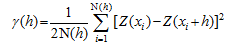
Table 1 The variogram fitting model and parameters of sediment combination
Sea area Combination Model Co Co+C Co/(Co+C) Ao (km) R2
LH Clay Line 5.4 132.3 0.041 10.8 0.978
Silt Spherical 33.5 301.3 0.111 23.9 0.970
Sand Spherical 62.0 728.0 0.085 24.1 0.973
AN Clay Spherical 41.6 115.7 0.360 51.0 0.833
Silt Gauss 93.5 387.9 0.241 24.0 0.982
Sand Gauss 208.0 826.9 0.252 23.7 0.970
AS Clay Exponential 5.2 43.5 0.120 9.3 0.880
Silt Gauss 0.1 58.4 0.002 4.3 0.791
Sand Gauss 0.1 132.5 0.001 4.7 0.850
The total spatial variability of each sediment particle in AS is smaller than that in LH and AN. The spatial variability of sand is the biggest and that of clay is the smallest in the study area, and the results indicate the sediment coarsening due to erosion. Spatial correlation is stronger in LH and AS, but weaker in AN, spatial autocorrelation ranges the smallest in AS (<10 km) to the largest in AN (up to 51 km). The values of Co/(Co+C) of clay and sand are less than that of silt in LH, indicating that the spatial autocorrelations of clay and sand are stronger than that of silt in LH. The spatial autocorrelation of silt is stronger in AN, whilst that of sand is stronger in AS. This spatial variability is closely related to the following influencing factors: the hydrodynamics is tide-dominant (tidal currents) and stable in LH and AS, but the effect of waves is significant and the wave-current interaction is complex in AN. The results also show that Ao changes less in LH than those in AS and AN, and the changes of Ao for clay is the biggest in all three areas because the dominant factor is tidal current.
In the large space of the study area, the dynamics of wave and tidal current which often control the spatial variability of the regional variables in different directions, results in the spatial variation showing distinct directional characteristics. In order to understand spatial variability of directional sedimentary characteristics, the semi-variances in two orthogonal groups of NE40˚/SE130˚ and E85˚/S175˚ are calculated, with their anisotropy ratios K(h) also being computed. When K(h) <1.0, it is isotropic and otherwise is anisotropy. Taking LH as an example (Figure 2), generally speaking, in the orthogonal directions of 85˚/175˚, there is a clear exhibition of anisotropy in the scale of 5 km, while in the scale larger than 5 km, it shows isotropy. In the orthogonal directions of 40˚/130˚, sediment composition shows anisotropy when the scale is larger than 7 km. This is due to flood-tidal currents directing to SW and ebb-tidal currents directing to NE. Different sized sediments were sorted and transported by the tidal currents in flood and ebb phases respectively. As a result, different sediment combinations are found to show different trends along current directions, which clearly shows anisotropy as seen in the orthogonal directions of 40˚/130˚. For a smaller scale, waves are found to have impacted on the surface sediments. Similar patterns can be seen in AN and AS: anisotropy beyond the scale of 8 km in K(h) 40˚/130˚and isotropic within 8 km in K(h) 85˚/175˚.
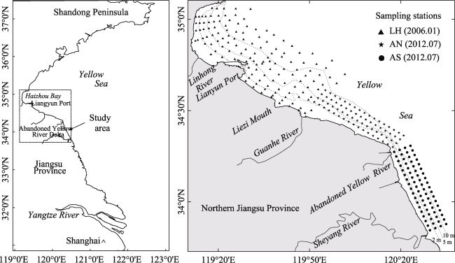
Figure 2 Ratios of anisotropic semivarigram of composition in LH
4.1.2 Sediment types
According to the classification of Folk (1970), sediment types in littoral area of the AYRD include: silty sand, sandy silt, silt, muddy sand, sandy mud and mud. A total of 6 types of sediments are found in LH, and 5 types of sediment are found in AN and AS, without the presence of mud (Figure 3). Sandy silt and silt are distributed widely and continuously, while mud and sandy mud appear to be patchily distributed. The overall trend of the plan distribution of sediments based on the median grain size is seen to vary from fine to coarse in the seaward direction in LH, while the sediment size changes from coarse to fine in the seaward direction in AN and AS. The characteristics of sediment distribution are found in a close relationship with hydrodynamics. Taking LH as an example, tidal currents become weak in the nearshore area, while waves and tidal currents are strong in the offshore area.
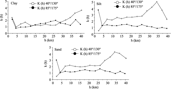
Figure 3 Sediments type of northern Jiangsu offshore

4.2 Characteristic distance (Dc)

Characteristic distance (Dc) is essential in the grain size trend analysis model: if Dc is less than the range of spatial autocorrelation, the adjacent points are less likely to cause information loss, and the trend vector cannot be sufficiently performed. On the contrary, if Dc is greater than the range of spatial autocorrelation, sufficient noise will be introduced, which will affect the authenticity of trend vector.
4.2.1 Maximum sampling intervals
As shown in Figure 1, the sampling stations are distributed quite regularly in the study area. The minimum and maximum sampling intervals in LH are 1.2 km and 8.7 km, respectively, with an average of 4.2 km, and Figure 4 shows the histogram of the sampling intervals. The average sampling intervals in both AN and AS are around 3 km, with a maximum of 3.1 km in AN and 3 km in AS. Setting initially the maximum sampling intervals as the Dc, the sediment trend vectors calculated based on the Gao and Collins method are shown in Figure 5, the results show that the sediment transport in LH are mainly in the direction towards the top of the Haizhou Bay, which is consistent with the sediment deposition found in the bayhead. However, the trend is unable to reflect the deposition in the southern part of the Haizhou Bay. Sediment transport trend is seaward at the Liezi Mouth and Guanhe Mouth, but is less clear in the offshore area of the LH. The sediment transport trends are non-conclusive in both AN and AS. Therefore, it can be concluded that to set the maximum sampling interval as Dc may be inadequate in the littoral area of the AYRD.
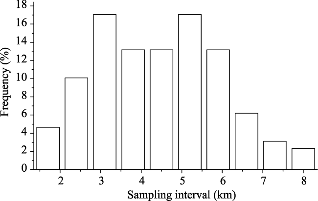
Figure 4 The samples' distances histogram for Lianyun Port sea area (LH)
4.2.2 Geostatistical Dc
The Kriging interpolation method is then used to obtain more regular grids of mean size, sorting coefficient and skewness. The semivariograms are subsequently calculated for Ao (Table 2), and a value between the minimum or the maximum sampling intervals is used as the interpolation radius. The results show that the semivariograms change with the increase of interpolation radius, and Dc has a great influence on sediment trend vectors. With averaging Ao of three parameters as Dc, the results of sediment transport are shown in Figure 6, indicating that different Dc can cause a significant change in sediment transport. When setting the average Ao of mean size as Dc, sediment transport vectors are in opposite to the residual current vectors at the Liezi Mouth. Similarly, it appears that with other average Ao, the southwest-northeast sediment transport vectors are in opposite to the southeast-northwest tidal currents in Haizhou Bay. Therefore, it becomes obvious that sediment transport trend calculated with this method cannot be reflected in AN and AS, either. Thus, the Dc obtained from preliminary interpolation is again unsuitable for sediment transport analysis in the study area.
Table 2 The range of the three parameters at different interpolating intervals before filtering (km)
Sea area Interpolating distance 1.0 2.0 3.5 5.0 7.0 Mean value
LH Mean size 42.1 41.3 42.1 41.5 34.7 40.3
Sorting 62.9 62.4 64.5 67.5 61.2 63.7
Skewness 32.6 32.9 33.1 34.0 31.9 32.9
Interpolating distance 1.0 1.9 3.0 3.5 4.2 Mean value
AN Mean size 22.4 22.7 23.9 21.6 23.2 22.7
Sorting 4.4 4.6 4.7 4.7 6.0 4.9
Skewness 28.0 28.3 31.6 25.2 28.1 28.3
AS Mean size 17.9 18.5 19.6 20.2 21.5 19.5
Sorting 17.0 17.7 19.1 18.5 19.7 18.4
Skewness 18.9 19.5 20.2 19.5 20.1 19.6
The reason for the deficiency of using Dc obtained by the preliminary interpolation is that the distance is beyond sediment spatial autocorrelation and considerable noise can be introduced. In order to search a better Dc, the filtering method is used to remove the data not at the sampling station and the filtered data are taken after the Kriging interpolation in semi-variance analysis to calculate Ao (Table 3). The sediment transport vectors calculated by Gao and Collins (1994) method are shown in Figure 6, the sediment transport vectors become much improved. Comparing the results with those obtained from the average values (Ao) of different parameters and hydrodynamics, it is clear that setting Ao to 26.0 km (LH), 39.9 km (AN) and 9.0 km (AS) respectively as the suitable Dc, the sediment transport vectors are well presented in the littoral area of the AYRD (Figure 5).
Table 3 The range of the three parameters at different interpolating intervals after filtering (km)
Sea area Interpolating distance 1.0 2.0 3.5 5.0 7.0 Mean value
LH Mean size 30.5 30.7 31.4 13.8 31.9 27.7
Sorting 36.9 36.2 35.2 34.6 31.3 34.8
Skewness 28.4 28.6 28.2 12.8 31.9 26.0

AN
Interpolating distance 1.0 1.9 3.0 3.5 4.2 Mean value
Mean size 55.6 54.5 29.0 43.3 17.0 39.9
Sorting 2.8 3.1 3.0 7.0 6.8 4.5
Skewness 9.5 10.0 19.2 7.1 7.9 10.8
AS Mean size 5.4 5.5 5.2 5.3 5.7 5.4
Sorting 5.4 13.7 5.3 5.2 5.3 7.0
Skewness 5.7 14.5 5.1 5.6 14.1 9.0
The above analysis shows that using different values of Dc in the grain size trend analysis model would induce different sediment transport patterns. Setting the maximum sampling interval as Dc, is unable to determine the relationship between sampling intervals and sediment transport patterns, and so is to generate satisfactory spatial correlation. However, the geostatistical method together with the filtering techniques can be used to improve the model accuracy and reproduce satisfactory sediment transport patterns in comparison with the field observations. By combining the hydrodynamics with different values of Ao, the model results reveal that the distances of 26.0 km (LH), 39.9 km (AN) and 9.0 km (AS) should be chosen as Dc in the grain size trend analysis model for the study site.
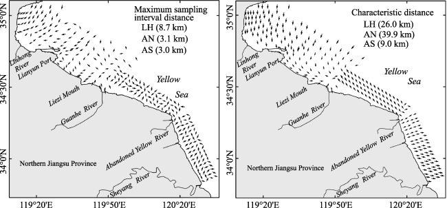
Figure 5 Sediments transport trend when using maximum sampling interval as Dc (left) and suitable Dc (right)
For this particular study area, we also find that there are certain patterns of linking Dc with Ao in different sediment combinations. The best Dc value for different areas is found to be close to the Ao of a certain sediment combination, for example, the Ao of sand in LH, and Ao of clay in AS, and the average Ao of three combinations in AN, close to Dc of each area. Therefore, determining Dc with the geostatistics model, the Ao of a particular type of sediment combination can be considered as Dc, as this can ensure the sediment spatial correlation. Using the values of Dc further away from the aforementioned will produce unrealistic sediment transport patterns as previously demonstrated.
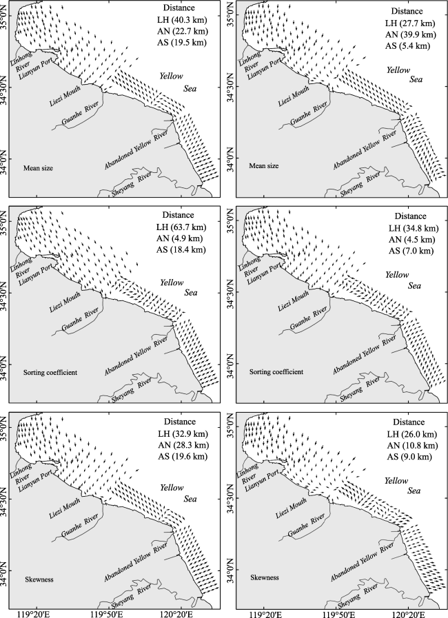
Figure 6 Sediment transport trend with mean range of the three parameters before filtering (left) and after filtering (right)

4.3 Sediment transport

Sediment transport trends shown in Figure 5 display that sediment is mainly transported towards the bayhead and south of the Haizhou Bay, which agrees with the hydrodynamic environment (Xie et al., 2007). In the area outside the Lianyun Port, the trends are found to be southeasterly in the nearshore area and southwesterly in the offshore area, which again agree well with the observed patterns. The sediment transport directions at the Liezi Mouth and Guanhe River coincide with the residual tidal currents, which is consistent with the results of the previous studies (Wang et al., 1980; Xie et al., 2008). Zhang (2013) also confirmed identical trends of sediment transport both in winter and summer seasons in LH. Sediment is transported to the northwest in AN, which is evidenced by the development direction of the sand spit at Guanhe River (Zhang and Zhang, 1993). The sediment transport trend is found to be southeasterly at the corner of the AYRD, offshore to the northern side of AS and southeasterly in the southern side of AS. Sediment transport trend in the nearshore area agrees with the residual currents in AS (Liu et al., 2012). In AS, the trends are found to rotate clockwise from the east to southeastwards. As agreed with other related studies (Wan and Zhang, 1985; Chen et al., 2011), we conclude that the sediment in this area is mainly transported towards the southeast and offshore.
Basically, sediment transport is the advection and diffusion process along the coast under varying hydrodynamics (Yun et al., 1981). Combined with wave, tide, current, runoff, and so on (Figure 7), sediment transports are analyzed. In the area where the water depth is shallower than 5 m, waves are the main dynamic forcing to cause morphological changes. In the area with water depth being between 5-10 m, the combined action of waves and tidal currents is dominated (Meng, 2000; Wang et al., 2011). Tidal currents rotate in the Lianyun Port (Chen, 2006), but the tides become reciprocating in the Haizhou Bay and AYRD. According to the work carried out by the Nanjing Hydraulic Research Institute (1993), sediment transport was southeasterly in the AYRD and AS, and northwesterly at the AN. On the other hand, residual currents are the main forcing to affect the grain size spatial variability (Ma et al., 2010). Finally, the Yellow Sea coastal currents (YSCC) exist along the Jiangsu coast (Wei et al., 2011; Yuan and Hsueh, 2010), and the sediment in the offshore area is mainly transported towards southeast under the influence of the YSCC. Due to the high concentration and a wide range of suspended sediments along AS, it can be expected that the sediment spreads in the offshore area (Xing et al., 2010). The above analysis shows that the skewness in both LH and AS, and the mean size in AN have the isotropic characteristics, which will assure the applicability of the grain size trend analysis model in the study area. Therefore, taking their average ranges (Ao) as the Dc in the grain size trend analysis model, the trends of sediment transport of the littoral area of the AYRD could be better represented, and the results are also supported by the results of previous research work and the hydrodynamic environment in the study area.

4.4 Coast evolution

Due to the Yellow River shifting to the north, the northern Jiangsu coasts had suffered continuous erosion, and the eroded sediment was transported to different areas by the hydrodynamic forcing (Figure 7). From 1960 to 2005, in the nearshore area of the Haizhou Bay, erosion occurred at the northern part and deposition at the southern part (Wang, 2006). The erosion-deposition at Lianyun Port was in a balance due to the rocky coastline. From the Lianyun Port to Zhongshan River Mouth, coastal erosion occurred (Wang, 2006), and sediment was mainly transported along the coastline. Erosion was relatively severe around the delta corner and southern sides of the AYRD, with sediment mainly being transported offshore. The above analysis shows that in the area, onshore sediment transport would result in deposition, and offshore sediment transport results in erosion in general.
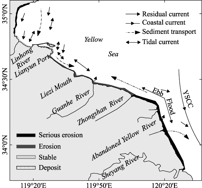
Figure 7 Condition of coastline erosion-deposition and dynamic environment (YSCC = Yellow Sea Coastal Current)

5 Conclusions

(1) Sediment variability characteristics are analyzed by the geostatistics analysis method in the littoral area of the AYRD on a macro scale. The results show that the sedimentary spatial correlation at Lianyun Port and AS is better than that at AN, and sediment appears to be anisotropy in the northeast-southeast direction. The sandy silt and silty sand are widely distributed in the study area, and grain size distributions are opposite in the nearshore area (fine-coarse) and offshore area (coarse-fine) in LH and the AYRD.
(2) When sediment transport is calculated using the grain size trend analysis model, it is found the simply using the maximum sampling intervals as Dc wouldn’t effectively reproduce a realistic trend of sediment transport. Using the geostatistics analysis method to determine Dc is an effective way to calculate the sediment transport trend vectors using the grain size trend analysis model, which could produce satisfactory sediment transport trends of surface sediments in the study area. Filtering method can effectively reduce the data noise so as to enhance accuracy of the data. At the same time, suitable Dc could provide guidance for designing sampling station of field investigation, and we believe that the sampling distance should be appropriately increased (e.g. 26.0 km in LH, 39.9 km in AN and 9.0 km in AS).
(3) The trends analysis of sediment transport shows that: sediment is transported to the top and south in the Haizhou Bay; to the outer channel in the Lianyun Port; to the southeast in nearshore and to the southwest in offshore along the coast in the south of Lianyun Port; to the offshore at Liezi Mouth and Guanhe River Mouth; and to the northwest in AN. It is also found that part of sediment is transported to southeast at the corner of the AYRD, and the change clockwise from the east to the southeast in AS. Sediment transport trends agree with the hydrodynamic forcing (circulation, tidal current, waves and residual current) and correlate to the nearshore topography evolution (accretion or erosion of coastline) in the study area.

The authors have declared that no competing interests exist.

1
Antunes Do Carmo J S, Seabra-Santos F J, 2002. Near-shore sediment dynamics computation under the combined effects of waves and currents.Advances in Engineering Software, 33: 37-48.

2
Balsam W L, Beeson J P, 2003. Sea-floor sediment distribution in the Gulf of Mexico. Deep Sea Research Part I:Oceanographic Research Papers, 50(12): 1421-1444.

3
Caeiro S, Painho M, Goovaerts Pet al., 2003. Spatial sampling design for sediment quality assessment in estuaries.Environmental Modelling & Software, 18: 853-859.

4
Chen Bin, Zhou Liangyong, Liu Jianet al., 2011. The relation between the suspended sediment movement and tidal current dynamic characteristic in Old Yellow River Delta.Marine Sciences, 35(5): 73-81. (in Chinese)

5
Chen Binlin, 2006. Environmental evolution and countermeasure research of Lianyungang offshore area. Shanghai: Dissertation for doctor degree of East China Normal University. (in Chinese)

6
Chen Kefeng, 2008. Research of land and ocean interactions progress of the coastal zone in Jiangsu Province since the Yellow River flows northward. Nanjing: Dissertation for doctor degree of Nanjing Hydraulic Research Institute. (in Chinese)

7
Cheng P, Gao S, Bokuniewicz H, 2004. Net sediment transport patterns over the Bohai Strait based on grain size trend analysis. Estuarine, Coastal and Shelf Science, 60(2): 203-212.

8
Dong L X, Guan W B, Chen Qet al., 2011. Sediment transport in the Yellow Sea and East China Sea. Estuarine,Coastal and Shelf Science, 93: 248-258.

9
Duman M, Avci M, Duman Set al., 2004. Surficial sediment distribution and net sediment transport pattern in Izmir Bay, western Turkey.Continental Shelf Research, 24(9): 965-981.

10
Fan S J, 2001. Coastal ocean morphodynamics and the resulting erosion and deposition: an analytical approach. USA: Dissertation for doctor degree of Old Dominion University.

11
Folk R L, Andrews P B, Lewis D W, 1970. Detrital sedimentary rock classification and nomenclature for use in New Zealand. New Zealand Journal of Geology and Geophysics, 13(4): 937-968.

12
Gao S, 2001. The use of grain size trends in marine sediment dynamics: A review.Chinese Journal of Oceanology and Limnology, 19(3): 265-271.

13
Gao S, 2009a. Modeling the preservation potential of tidal flat sedimentary records, Jiangsu coast, eastern China.Continental Shelf Research, 29: 1927-1936.

14
Gao S, 2009b. Grain size trend analysis: Principle and applicability.Acta Sedimentologica Sinica, 27(5): 826-836. (in Chinese)

15
Gao S, Collins M, 1991. A critique of the McLaren Method for defining sediment transport paths: Discussion.Journal of Sedimentary Petrology, 61(1): 143-146.

16
Gao S, Collins M, 1992. Sand sediment transport patterns inferred from grain-size trends based upon definition of “transport vectors”.Sedimentary Geology, 80(1/2): 47-60.

17
Gao S, Collins M, 1994a. Analysis of grain size trends, for defining sediment transport pathways in marine environments.Journal of Coastal Research, 10(1): 70-78.

18
Gao S, Collins M, 1994b. Net sediment transport patterns inferred from grain-size trends, based upon definition of ‘transport vectors’: Reply.Sedimentary Geology, 90: 157-159.

19
Liu T, Shi X F, Li C Xet al., 2012. The reverse sediment transport trend between abandoned Huanghe River (Yellow River) Delta and radial sand ridges along Jiangsu coastline of China: An evidence from grain size analysis.Acta Oceanologica Sinica, 31(6): 83-91.

20
Ma F, Wang Y P, Li Yet al., 2010. The application of geostatistics in grain size trend analysis: A case study of eastern Beibu Gulf.Journal of Geographical Sciences, 20(1): 77-90.

21
Matheron G, 1963. Principles of geostatistics. Economic Geology, 58: 1246-1266.

22
Mc Laren P, 1981. An interpretation of trends in grain size measures.Journal of Sedimentary Petrology, 51(2): 611-624.

23
Mc Laren P, Bowles D, 1985. The effects of sediment transport on grain-size distributions.Journal of Sedimentary Petrology, 55(4): 457-470.

24
McManus J, 1988. Grain size determination and interpretation. In: Tucher M (ed.). Techniques in Sedimentology. Oxford: Blackwell, 63-85.

25
Meng Qinghai, 2000. Geomorphic evolution and trend of abandoned delta: Focus on abandoned Yellow River Delta of north Jiangsu Province. Shanghai: Dissertation for doctor degree of East China Normal University. (in Chinese)

26
Murraya C J, Leeb H J, Hampton M A, 2002. Geostatistical mapping of effluent-affected sediment distribution on the Palos Verdes shelf.Continental Shelf Research, 22: 881-897.

27
Nanjing Hydraulic River-Port Research Institute, 1993. Hydrogeological investigation and data analysis of Binhai Seas field. (in Chinese)

28
Peng Jun, Chen Shenliang, 2010. Response of delta sedimentary system to variation of water and sediment in the Yellow River over past six decades.Journal of Geographical Sciences, 20(4): 613-627.

29
Poizot E, Mear Y, Thomas Met al., 2006. The application of geostatistics in defining the characteristic distance for grain size trend analysis.Computers & Geosciences, 32: 360-370.

30
Ren Mei’e, 1985. Coastal and Tidal Flat Resources Investigation of Jiangsu Province. Beijing: China Ocean Press. (in Chinese)

31
Roux J P, O’Brien R D, Rios Fet al., 2002. Analysis of sediment transport paths using grain-size parameters.Computers & Geosciences, 28: 717-721.

32
Wan Yanshen, Zhang Qinian, 1985. The source and movement of sediments of radiating sand ridges off Jiangsu coast.Oceanologia et Limnologia Sinica, 16(5): 392-399. (in Chinese)

33
Wang Baochan, Yu Zhiying, Liu Cangzhiet al., 1980. The change of coasts and beaches and the movement of longshore sediments of Haizhou Bay.Acta Oceanologica Sinica, 2(1): 80-96. (in Chinese)

34
Wang X H, Qiao F L, Lu Jet al., 2011. The turbidity maxima of the northern Jiangsu shoal-water in the Yellow Sea, China.Estuarine, Coastal and Shelf Science, 93: 202-211.

35
Wang X Y, Ke X K, 1997. Grain-size characteristics of the extant tidal flat sediments along the Jiangsu coast, China.Sedimentary Geology, 112: 105-122.

36
Wang Yanhong, 2006. Study of variation features during coastal erosion processes on the Abandoned Huanghe River Delta and integrated protection measures. Nanjing: Dissertation for doctor degree of Nanjing Normal University. (in Chinese)

37
Wang Y P, Gao S, Jia J Jet al., 2012. Sediment transport over an accretional intertidal flat with influences of reclamation, Jiangsu coast, China. Marine Geology, 291-294: 147-161.

38
Wang Zhengquan, 1999. Statistics and Application in Ecology. Beijing: Science Press, 59-149. (in Chinese)

39
Wei Qinsheng, Yu Zhigang, Ran Xiangbinet al., 2011. Characteristics of the western coastal current of the Yellow Sea and its impacts on material transportation.Advances in Earth Science, 26(2): 145-156. (in Chinese)

40
Xie Fei, Pang Yong, Song Zhirao, 2007. Three-dimensional numerical simulation of tidal current in offshore area of Haizhou Bay. Journal of Hohai University (Natural Sciences), 35(6): 718-721. (in Chinese)

41
Xie Fei, Pang Yong, Zhuang Weiet al., 2008. Study on regularity of matter transportation in the nearshore area of the Haizhou Bay.Advances in Marine Science, 26(3): 347-353. (in Chinese)

42
Xing Fei, Wang Yaping, Gao Jianhuaet al., 2010. Seasonal distributions of the concentrations of suspended sediment along Jiangsu coastal sea.Oceanologia et Limnologia Sinica, 41(3): 459-468. (in Chinese)

43
Yuan D L, Hsueh Y, 2010. Dynamics of the cross-shelf circulation in the Yellow and East China Sea in winter. Deep-Sea Research II, 57: 1745-1751.

44
Yun Caixing, Cai Mengyi, Wang Baoquan, 1981. An analysis of the diffusion of suspended sediment discharged from the Changjiang River based on the satellite images.Oceanologia et Limnologia Sinica, 12(5): 391-401. (in Chinese)

45
Zhang Chunyong, 2013. Sediment transport trend in Lianyungang nearshore area.Acta Oceanologica Sinica, 35(3): 172-178. (in Chinese)

46
Zhang Dongsheng, Zhang Changkuan, 1993. Dynamic analysis of estuarine deposition in Guanhe estuary.Journal of Hohai University, 21(4): 29-37. (in Chinese)

47
Zhang Yong, Swift Donald J Pet al., 1998. Modeling of coastal profile evolution on the abandoned delta of the Huanghe River. Marine Geology, 145: 133-148.

48
Zhao Lirong, 2010. Spatial variability of soil nutrients under different parent materials. Chongqing: Dissertation for master degree of Southwest University. (in Chinese)

Outlines

/