Research Articles

Spatiotemporal dynamics of carbon intensity from energy consumption in China

  • CHENG Yeqing , 1 ,
  • WANG Zheye 1, 2 ,
  • YE Xinyue 3 ,
  • WEI Yehua Dennis 4
Expand
  • 1. Northeast Institute of Geography and Agroecology, CAS, Changchun 130102, China
  • 2. University of Chinese Academy of Sciences, Beijing 100049, China
  • 3. Department of Geography, Kent State University, Kent, Ohio 44242, USA
  • 4. Department of Geography, University of Utah, Salt Lake City, UT 84112-9155, USA

Author: Cheng Yeqing (1976-), PhD and Associate Professor, specialized in economic geography and rural development. E-mail:

Received date: 2013-10-27

  Accepted date: 2013-12-05

  Online published: 2014-04-20

Supported by

Key Research Program of the Chinese Academy of Sciences, No.KZZD-EW-06-03.No.KSZD-EW-Z-021-03.Key Project of Chinese Ministry of Education, No.13JJD790008.National Natural Science Foundation of China, No.41329001.No.41071108

Copyright

Journal of Geographical Sciences, All Rights Reserved

Abstract

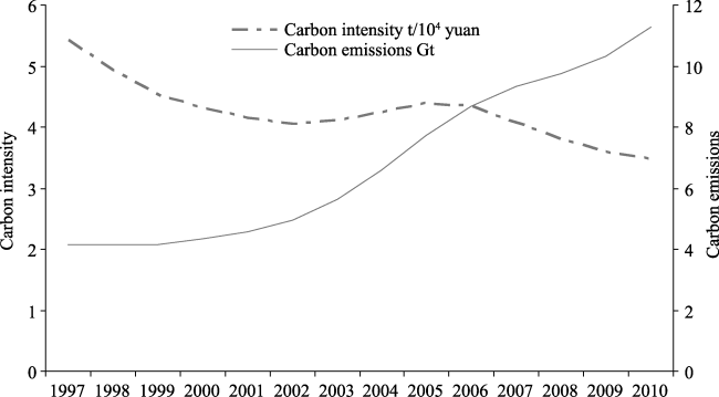
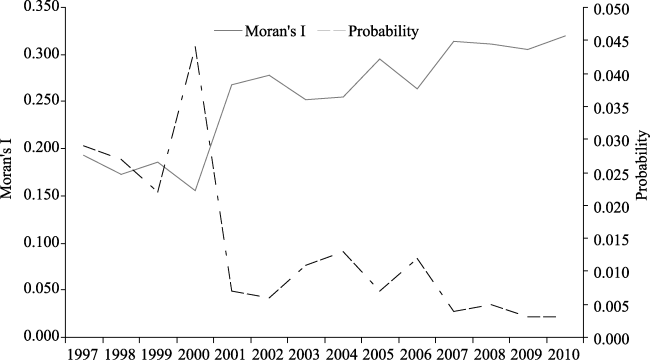
The sustainable development has been seriously challenged by global climate change due to carbon emissions. As a developing country, China promised to reduce 40%-45% below the level of the year 2005 on its carbon intensity by 2020. The realization of this target depends on not only the substantive transition of society and economy at the national scale, but also the action and share of energy saving and emissions reduction at the provincial scale. Based on the method provided by the IPCC, this paper examines the spatiotemporal dynamics and dominating factors of China’s carbon intensity from energy consumption in 1997-2010. The aim is to provide scientific basis for policy making on energy conservation and carbon emission reduction in China. The results are shown as follows. Firstly, China’s carbon emissions increased from 4.16 Gt to 11.29 Gt from 1997 to 2010, with an annual growth rate of 7.15%, which was much lower than that of GDP (11.72%). Secondly, the trend of Moran’s I indicated that China’s carbon intensity has a growing spatial agglomeration at the provincial scale. The provinces with either high or low values appeared to be path-dependent or space-locked to some extent. Third, according to spatial panel econometric model, energy intensity, energy structure, industrial structure and urbanization rate were the dominating factors shaping the spatiotemporal patterns of China’s carbon intensity from energy consumption. Therefore, in order to realize the targets of energy conservation and emission reduction, China should improve the efficiency of energy utilization, optimize energy and industrial structure, choose the low-carbon urbanization approach and implement regional cooperation strategy of energy conservation and emissions reduction.

Cite this article

CHENG Yeqing , WANG Zheye , YE Xinyue , WEI Yehua Dennis . Spatiotemporal dynamics of carbon intensity from energy consumption in China[J]. Journal of Geographical Sciences, 2014 , 24(4) : 631 -650 . DOI: 10.1007/s11442-014-1110-6

1 Introduction

With the rapid propulsion of industrialization and urbanization, global warming has become one of the most serious challenges to sustainable development, which is usually attributed to greenhouse gas emissions from traditional fossil-fuel energy consumption (IPCC, 2007; Zhao et al., 2011; Chuai et al., 2012a). Therefore, addressing climate change and reducing carbon emissions has become a global issue that attracts increasing attentions from both the policy makers and scholars, and developing low-carbon economy has thus become a worldwide consensus (Liu et al., 2008; Chuai et al., 2012b; Lu et al., 2012). As a developing country, China has been experiencing a gradual transition from a planned economy to a market economy, has achieved spectacular economic growth in the last three decades (Li and Wei, 2010). It has led to a long-term and higher-speed growth of energy consumption, as well as the carbon emissions. The gross energy consumption in China accounts for 20% of global primary energy consumption, and 90% of China’s carbon emissions are from the combustion of fossil-fuel energy. China’s carbon emission has attracted concerns from the western countries, which ask China to undertake a larger share of carbon emissions reduction. China has surpassed the United States and become the leading country in CO2 emissions in the world (IEA, 2009). Moreover, due to the long-term durative influence of economic growth and industrial transition, China’s CO2 emissions will increase unceasingly, leading to increasing diplomatic pressure in international climate negotiation on combating with global climate change (Zhang, 2010). In this context, China pledged to reduce carbon intensity by 40%-45% below the 2005 level by 2020 to reach the international climate agreement in Copenhagen. In addition, carbon intensity has been included in the long-term planning of China’s socioeconomic development, indicating that China’s energy policy will face a strategic transition from emphasizing energy efficiency to improving energy structure. Meanwhile, the realization of this target depends on not only the substantive transition of socioeconomic structure at the national level, but also the action and share of energy saving and emissions reduction at the provincial level. However, China is a nation with vast territory, where remarkable differentiation exists in resources endowment, population scale, economic development level, industrial structure, and energy consumption structure. Therefore, national energy saving and carbon emission reduction can only be realized by allocating share of carbon emission reduction and implementing differential policies.
Carbon intensity (CI) is defined as the ratio of carbon emissions to the gross domestic products (GDP). Low carbon intensity indicates that a country or a region is able to produce each unit of output with fewer carbon emissions. Carbon intensity is used as one of the most important indicators to measure energy utilization quality and carbon emission efficiency. Moreover, increasing literatures have attempted to describe and explain these dynamic patterns and factors from different perspectives. Most studies agreed that energy intensity and energy structure are the two uppermost factors affecting carbon intensity. For example, Greening et al. (1998, 1999, 2001 and 2004) examined the carbon intensity in 100 OECD countries using adaptive weighted division index (AWD) and argued that energy intensity of the production sector was the main factor. Schipper et al. (2001) analyzed the carbon intensity of nine manufacturing sectors in 13 IEA countries using factor decomposition method and explained the dominating factors of carbon emission declining. Obas and Anthony (2006) decomposed CO2 emission intensity of some African countries and considered that energy intensity, energy type and economic structure are the dominating factors that influence carbon intensity. Bhattacharyya et al. (2010) found that the declining of carbon intensity in the EU-15 came mainly from Germany and UK, and the declining of energy intensity is the decisive factor. Simone et al. (2011) had a contrastive analysis of carbon intensity of Austria and Czech using the methods of Kaya identical equation and logarithmic comparison and found that both the energy intensity and industrial structure have important influence on carbon intensity. However, Nag and Parikh (2000) argued that the growth of income per capita is the main factor causing the increase of carbon intensity, and there exists an inverse U-shaped relationship between carbon emissions and income per capita (Ang et al., 2006), while Davis et al. (2003) considered that climate change is the uppermost factor that causes the declining of energy intensity and carbon intensity from 1996 to 2000, instead of energy structure adjustment. But on how to reduce carbon intensity, scholars have different viewpoints. David et al. (2011) argued that biomass fuel and hydrogen power vehicle are the key to reduce carbon intensity from transport in the future 50 years, and it is still a difficult issue in future studies to search for stable and sustainable cleaning energy to replace the fossil energy. Simone et al. (2010) argued that biomass energy plays a more important role in energy balance and carbon intensity reduction. Besides, after analyzing the influence of input-output ratio, temperature and technique on energy intensity, Stem et al. (2010) forecasted the tendency of carbon intensity in China and India and indicated that it is more difficult for China to realize the carbon emission reduction target. Therefore, more radical policies should be implemented in China for future sustainable development.
Since the Central Government of China pledged the target of carbon emission reduction in 1999, concerns about China’s carbon intensity have been raised worldwide and studies have been done utilizing different data sources and methodologies. Yue et al. (2010) and Tan and Huang (2008) analyzed the carbon intensity in China using Theil`s index based on the data from the Oak Ridge National Laboratory, and found that western China has a higher carbon intensity than eastern China. Sather et al. (2011) examined the eastern, central and western regions using the variable coefficient, Gini coefficient and Theil’s index, and argued that no significant regional difference existed. Yang and Liu (2012a) conducted a structural decomposition of carbon intensity for the eastern, central, western and northeastern China, and found that regional difference is generated mainly by the four inland regions. Besides, Zhao et al. (2011) analyzed the spatiotemporal patterns of China’s carbon intensity in 1997-2007 utilizing spatial autocorrelation analysis and argued that carbon intensity in provincial China demonstrated positive spatial agglomeration. The ‘cold spot’ areas were concentrated mainly in the coastal regions with a relative steady situation, while the ‘hot spot’ areas transferred from Northwest China to the middle Yellow River Basin and Northeast China. In addition, Yao and Ni (2011) argued that foreign direct investment (FDI) can reduce regional carbon intensity effectively. Ying et al. (2007) analyzed the factors affecting China’s carbon intensity using adaptive weighted logarithmic index and indicated that energy structure and energy intensity are the decisive factors on carbon intensity. Du (2010) argued that the proportion of heavy industry, urbanization level and the proportion of coal consumption have significant positive influence on China’s CO2 emissions, and there exists an inverse U-shaped relationship between economic development level and per capita CO2 emissions. Wu et al. (2011) established an optimized model of per capita carbon emission, per capita income, urbanization rate and the proportion of service, and classified the 112 self-governed economic units into four stages and five typical modes. Yang and Liu (2012b) indicated that energy intensity, energy structure, per capita GDP and industrial structure have decisive impact on carbon intensity.
However, it should be noted that most econometric methods in the above studies depended mainly on the theoretical hypotheses of traditional statistics, which treated the spatial units as independent and homogeneous individual and tended to ignore the spatial relationships among spatial units. According to Tobler’s first law of geography, all values on a geographic surface are related to each other, and closer observations are more strongly related than distant ones (Tobler, 1970). Spatial autocorrelation analysis can reflect the spatial relationships between any focal spatial unit and its neighbors based on spatial weight matrix (Cliff and Ord, 1981), therefore, it can be applied to illustrate the spatial correlative degree of carbon intensity and reveal its spatial distribution patterns. Spatial panel econometric model elucidates the specific impact of the selected factors by nesting temporal and spatial effects (Anselin, 1988). However, to date many panel data models ignored spatial interaction (Ye and Wu, 2010). This paper attempts to examine the spatiotemporal patterns of China’s carbon intensity from energy consumption using the spatial autocorrelation analysis, and explain the dominating factors through spatial panel econometric model. In addition, the authors propose some suggestions from the perspective of fossil energy utilization and structural adjustment of energy consumption. The aim is to provide a scientific basis for China to implement differential policies and strategies of energy saving and carbon emission reduction as well as the share of carbon reduction among provinces.

2 Method and data

2.1 Carbon intensity model

CO2 emissions come mainly from the combustion of fossil energy, which are estimated according to the energy consumption. Based on the method provided by the Intergovernmental Panel on Climate Change (IPCC, 2006), the CO2 emissions are estimated by calculating the product of the total consumptions, average low-order calorific value and the CO2 emission coefficients of eight types of fossil energy such as natural gas, diesel oil, coal oil, gasoline, fuel oil, crude oil, coke and coal (Table 1). The equation is given as:
where CE denotes the total CO2 emissions, NCVi refers to the average low-order calorific value of each type of fossil energy, which can be derived from the appendix 4 of the China Energy Statistical Yearbook 2011; CEFi denotes the CO2 emission coefficients of the ith energy provided by the IPCC (Table 1).
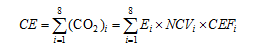
Table 1 Average low-order calorific value and the CO2 emissions coefficient of each kind of fossil energy
Natural gas Diesel oil Coal oil Gasoline Fuel oil Crude oil Coke Coal
NCV 38931 42652 43070 43070 41816 41816 28435 20908
CEF 56100 74100 71500 70000 77400 73300 107000 95333
Based on total CO2 emissions and GDP in provincial China, the carbon intensity can be calculated with the following model:
where CIj denotes carbon intensity of the jth province, j refers to a specific province, with j = 1, 2, 3… 30.

2.2 Exploratory spatial data analysis (ESDA)

ESDA is a set of methods aiming at describing and visualizing geographical distributions. ESDA can be utilized to detect spatial outliers or atypical localizations, identify patterns of spatial association and indicate forms of spatial heterogeneity (Grubesic and Mack, 2008; Haining, 1990, Anselin, 1999). ESDA provides measures of global and local spatial autocorrelation to characterize the spatial distribution of a set of values (Ye and Wu, 2010). It is considered as a descriptive step before hypothesis test and regression model implementation (Anselin, 2005). Global autocorrelation is assessed by Global Moran’s I statistics. A positive and significant Moran’s I value indicates a general pattern of spatial clustering of similar values. Local indicator spatial autocorrelation (LISA) considers spatial proximity of each unit/value, which can identify the spatial hot spots of values (Anselin, 1995). The rapid development of new ESDA methods has stimulated a number of research efforts to analyze the spatial inequality and regional dynamics (Goodchild, 2006; Rey and Ye, 2010; Gallo and Ertur, 2003; Rey, 2004; Pu et al., 2005, Rey, 2001, Vilalta, 2010; Tu et al., 2012; Cheng et al., 2013; Ma et al,., 2013). This paper attempts to illustrate the spatiotemporal dynamics of China’s carbon intensity from 1997 to 2010.
2.2.1 Global spatial autocorrelation
Global Moran’s I is applied to detect the spatial autocorrelation and analyze spatial relationships among regions (Upton and Fingleton, 1985; Aneslin, 1988, 1995, 1996). An increasing Global Moran’s I indicates the growing convergence, while a decreasing Global Moran’s I reveals a more even spatial distribution (Yu and Wei, 2003).
Global Moran’s I is given as:
where n is the total number of the provinces; yi and yj denote the carbon intensity of the ith and jth province, respectively; ȳ is the average carbon intensity of the provinces; Wij is the binary weight matrix of the general cross-product statistic, in which the K-Nearest Neighbor is selected on the basis of the adjacency relations, and K fetches the accepted value of 4 to ensure each province has one neighbor at least. The z value is used to test the Global Moran’s I, which is given as:
where, if Z value is greater than 0 and significant in statistic, it indicates that there exists an obvious positive autocorrelation in spatial distribution of carbon intensity.
2.2.2 Local spatial autocorrelation
Global Moran’s I reveals overall spatial associations, but does not illustrate spatial association of individual units. To address this issue, we apply local spatial autocorrelation to undertake a disaggregated analysis of China’s carbon intensity. In the Moran scatterplot, the four different quadrants divide such two types of spatial association as the positive and negative associations into four types of local spatial association between individual provinces. Namely, High-High (quadrant I, positive associations) indicates high values surrounded by high values; Low-Low (quadrant III, positive associations) indicates low values surrounded by low values; Low-High (quadrant II, negative associations) and High-Low (quadrant IV, negative associations) indicate low values surrounded by high values, and high values surrounded by low values, respectively (Yu and Wei, 2003).

2.3 Spatial panel econometric model

Generally speaking, panel data covers a large amount of information and includes more changes and weaker co-linearity of variable, which can provide a higher freedom degree and improve the reliable estimates of the coefficients (Ji et al., 2011; Elhorst, 2003). Due to the spatial autocorrelation (spatial dependence) of carbon intensity among the provinces in each time section, the spatial panel econometric mode, based on the common panel data model and blended in spatial and temporal effect, can be applied to illustrate the driving mechanism of these selected factors on the spatiotemporal dynamic patterns of China’s carbon intensity.
2.3.1 Three models
Three types of spatial econometric models are usually applied to analyze the spatial interaction of dominating factors among study units, namely, spatial lag model (SLM), spatial error model (SEM) and spatial Durbin model (SDM), which are corresponded with different setting modes of spatial interaction (Lesage and Pace, 2009).
The SLM places more emphasis on the spatial correlation of the variables among the geographical units and inspects its spatial spillover effect. If the spatial interaction or spatial autocorrelation comes from the material correlation of regional trade, labor, capital, technology and knowledge flow, it can be analyzed by spatial lag factors including dependent variables (Hong et al., 2010). The equation is given below:
where i is an index of the cross-sectional spatial units, with i=1,, n, 30 provinces serve as the cross-sectional spatial units; the index of t represents the temporal periods, with t=1, …, T, and the three years are considered as three time points of temporal dimension (1997, 2000, 2010); δ is the spatial autoregressive coefficient; yit is an observation on the dependent variable (carbon intensity) at spatial unit i and time t; xit is a (1, k) row vector of observed value of independent variable at i and t; β is a matching (k, 1) of fixed but unknown parameters; μi denotes a spatial fixed effect, which controls all of the spatial fixing and the variables that will not change with time; λt denotes a time fixed effect, which controls all of the time fixing and the variables that will not change with space; wij is an element of a spatial weight matrix w, and w describes the spatial arrangement of all the spatial units in the sample.
The SEM inspects mainly the influencing degree of variable error on observation values. Some independent variables, which are relative to the dependent variable, have spatial autocorrelation, may be missed when we establish the spatial regression model, and the random error may influence the spatial spillover effect, for example, the elemental fluctuation of a spatial unit will spread to other regions through spatial transmission mechanism, therefore, spatial autocorrelation that ignores the error may lead to a bias when we establish the model under some condition. The equation is given as:
where ϕit denotes an error item of spatial autocorrelation; ρ is called a spatial autocorrelation coefficient of an error item (Elhorst, 2003, 2010).
The SDM combines the characters of SLM and SEM. It can inspect the spatial effect and influence of variable error on observation values, then achieves a better estimation effect (Lesage and Pace, 2009). The advantage of SDM is that spatial modes of the data may be explained with not only endogenous interaction or disturbance item, but also endogenous interaction, exogenous interaction and the autocorrelation of error item as well (Elhorst, 2003). The SDM is given as:
where γ is a matching (k, 1) vector of the parameters of spatial lag variables.
2.3.2 Estimation
According to the model proposed by Elhorst, two issues should be solved when the estimation and test are conducted: which spatial panel model to be selected and what kind of fixed effect to be included (Elhorst, 2010). Firstly, we should estimate and test the traditional mixed panel data model without regard to spatial interaction, and then test the spatial autocorrelation of the residual error to decide which one is more suitable to describe the data between the SLM and SEM and what kind of fixed effect should be included. Generally speaking, the OLS is usually applied to estimate the non-space panel data model, and the LMlag, LMerror, R-LMlag and R-LMerror are commonly applied to test the spatial autocorrelation of the residual error (Lesage and Pace, 2009), and the likelihood is usually used to test the fixed effect. Additionally, besides the traditional fitting goodness (R2) and Log Likelihood ratio, the Corrected R2 that ignores the influence of fixed effect is also applied to test the spatial panel model.
Secondly, we should analyze if the SDM can be simplified to SLM or SEM, the null hypothesis that can be simplified to SEM and SLM are H0: γ+δβ=0 and H0: γ = 0, respectively, both of which will be refused if the results pass through the test of 5% significant levels by the methods of Wald or likelihood ratio. Generally speaking, the maximum likelihood ratio is usually applied to estimate the parameters of SDM.
Finally, Lesage and Pace (2009) once argued that it may lead to wrong conclusion using the method of point estimation to test the existence of spatial spillover effect in the spatial regression model. Therefore, the partial differential equation should be applied to test the direct effects and spatial spillover effects of the variables on the basis of section model. Moreover, Elhorst applied this method to spatial panel model and illustrated its principle by taking the SDM as an example (Elhorst, 2010). The SDM can be rewritten to the vector quantity as:
where the error item of ε*t includes εt and fixed effect. Taking the derivative of the above equation with the kth explanatory variable, the partial differential matrix can be achieved as:
where the direct effect is defined as the mean value of the elements in principal diagonal of the matrix, reflecting the marginal effect of k variable to dependent variable of the section unit, and indirect effect is defined as the mean value of the elements except principal diagonal of the matrix, reflecting the marginal effect of k variable of one section unit to the dependent variables of other section units or the influence of k variable of other section units to the dependent variables of one section unit.

2.4 Data sources and variables

2.4.1 Spatial units
Our study consists of 30 provincial units, including 21 provinces and four municipalities directly under the Central Government of China and five Autonomous Regions, but Taiwan Province, the Hong Kong and Macao Special Administrative Regions and the Tibetan Autonomous Region are not covered for lacking of statistical data.
2.4.2 Data sources
Data of the total consumptions of natural gas, diesel oil, coal oil, gasoline, fuel oil, crude oil, coke and coal are from the China Energy Statistical Yearbook (NBSC, 1998-2011a); and the average low-order calorific values of each kind of fossil energy are derived from the appendix 4 of the China Energy Statistical Yearbook 2011; and the carbon emission coefficients of all kinds of fossil energy are derived from 2006 IPCC Guidelines for National Greenhouse Gas Inventories (IPCC, 2006); besides, data of gross domestic product (GDP) over these years are from the China Statistical Yearbook (NBSC, 1998-2011b) and are converted into the constant prices of the year 1997 based on the provincial implicit GDP. The GIS maps (shape files) are downloaded from China Data Center (http://chinadatacenter.org).
2.4.3 Variables
As many scholars argued (Greening et al., 1998, 1999, 2001, 2004; Schipper et al., 2001; Obas and Anthony, 2006; Yao and Ni, 2011), carbon intensity is an integrative concept and influenced by such factors as energy intensity, energy structure, economic development level, technical level and population, etc., which have different effects on and contributions to carbon intensity. In this paper, based on the literatures (Yang and Liu, 2012b; He and Zhang, 2006), eight explanation variables are selected to explain the spatial interaction mechanism of China’s carbon intensity. Almost all of the data of these variables are derived from the China statistical yearbook and China energy statistical yearbook in 1998-2011 except the data of FDI, which are from the Ministry of Commerce of China. The variables are explained as follows: 1) Total population (TP) is the arithmetic average of a year and the following year; 2) GDP per capita (GDPC) denotes the ratio of GDP and the total population; 3) Energy intensity (EI) refers to the ratio of total energy consumptions and GDP; 4) Energy structure (ES) denotes the proportion of coal consumptions to overall energy consumptions; 5) Industrial structure (IS) denotes the proportion of the output value of the secondary industry to GDP; 6) Urbanization rate (UR) refers to the ratio of non-agricultural population and the total population; 7) Foreign trade openness (FTO) refers to the proportion of total import-export volume to GDP; 8) Foreign direct investment (FDI) denotes the ratio of the total amount of FDI and GDP.

3 Findings and interpretations

3.1 Temporal characteristics

Figure 1 shows that the carbon emissions from energy consumption in China increased uninterruptedly from 4.16 Gt to 11.29 Gt (1 Gt = 109 t) in 1997-2010, with an annual rate of 7.15%, while the average growth rate of GDP was 11.72% (calculated by 1997 constant prices), which is much higher than that of the total CO2 emissions. Therefore, though the CO2 emissions increased year by year, the carbon intensity still showed a declining tendency from 5.43 t/103 yuan to 3.49 t/103 yuan in this period.
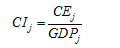
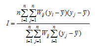
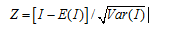
Figure 1 Carbon emissions and carbon intensity in 1997-2010
With the aid of GeoDa, the Global Moran’s I of China’s carbon intensity from energy consumption in 1997-2010 is calculated (Figure 2), and the significances of which are also tested by establishing the normal distribution with the method of random permutation. Figure 2 shows that all of the Moran’s I over these years were positive and the normal statistics z of annual Moran’s I passed through the 5% level of significance test, which indicated that China’s carbon intensity had significant spatial autocorrelation at the provincial scale during the study period, that is, the provinces with higher or lower carbon intensity tended to be adjacent. Meanwhile, Figure 2 shows that the Moran’s I of carbon intensity had a decreasing tendency with a small fluctuation from 1997 to 2000, with about 0.3 of stable concomitant probability, which indicated that the cluster degree of China’s carbon intensity had a slight decreasing tendency; while the Moran’s I increased significantly with a small fluctuation from 2000 to 2010, and the concomitant probability also decreased significantly compared with the previous period, which indicated that the spatial agglomeration of carbon intensity tended to be increasing significantly. As a whole, the agglomeration degree of China’s carbon intensity at the provincial scale has been strengthened since 1997 and the provinces with similar carbon intensity tended to be agglomerated in spatial distribution with a reduction.Spatial analysis is important to illustrate the spatial dynamic patterns of China’s carbon intensity. Therefore, according to the temporal characteristics of Moran’s I, three sectional estimation values of carbon intensity in 1997, 2000 and 2010 are selected to classify China’s 30 provinces into five grades (Figure 3), respectively.
Figure 2 Moran’s I of carbon intensity in 1997-2010

3.2 Spatial dynamics

As shown in Figure 3, the spatial distribution of China’s carbon intensity had obvious difference at the provincial scale that carbon intensity of the northern provinces was much higher than that of the southern provinces. In 1997, Shanxi and Guizhou provinces had the highest carbon intensity, and other northern and northeastern provinces such as Xinjiang, Gansu, Inner Mongolia, Ningxia, Liaoning and Jilin ranked the second place, while carbon intensity of the eastern coastal provinces such as Hainan, Zhejiang, Fujian, Guangdong and Guangxi were much lower than that of the above regions. In 2000, Shanxi became the province with the highest carbon intensity, and Inner Mongolia, Ningxia and Guizhou ranked second, while such provinces as Hunan and Jiangsu belonged to the group of lower carbon intensity. However, the spatial pattern of China’s carbon intensity had not changed radically,
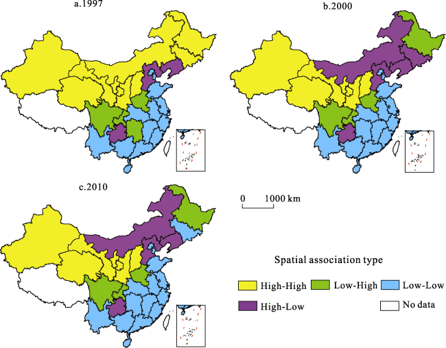
Figure 3 Spatial pattern of China’s carbon intensity in 1997, 2000 and 2010
that is, carbon intensities of the northern provinces were still higher than those of the southern provinces. In 2010, Ningxia became the province with the highest carbon intensity, and Guizhou and Shanxi ranked the second place. Moreover, the provinces with lower carbon intensity increased largely in this period, including such inland provinces as Jiangxi, Hubei, Sichuan and Chongqing, and in terms of China’s carbon intensity, it is clear that the northern provinces had higher values than the southern provinces.
After statistically analyzing the provincial change of China’s carbon intensity among the five grades (Table 2), we can find that regional patterns of China’s carbon intensity changed greatly in 1997-2010. For example, the proportion of the provinces that carbon intensity was between 3 and 14 decreased from 76.7% in 1997 to 70.0% in 2000 and 53.3% in 2010, and the provinces where carbon intensity was greater than 14 remained almost unchanged, while the proportion of the provinces where carbon intensity was below 3 increased from 16.7% in 1997 to 23.3% in 2000 and 43.3% in 2010. Therefore, the decrease of the provinces with higher carbon intensity and the substantial increase of the provinces with lower carbon intensity further evidenced the objective fact that China’s carbon intensity from energy consumption has been in a continuous decline since 1997.
Table 2 The provincial change of carbon intensity in 1997, 2000 and 2010
CI Provinces
1997 2000 2010
1-3 Zhejiang, Fujian, Hainan, Guangdong, Guangxi Jiangsu, Hunan, Hainan, Fujian, Guangdong, Zhejiang, Guangxi Beijing, Tianjin, Jiangsu, Sichuan, Hubei, Zhejiang, Chongqing, Guangxi, Fujian, Hunan, Hainan, Shanghai, Jiangxi, Guangdong
3-5 Shandong, Henan, Jiangsu, Anhui, Hubei, Hunan, Sichuan, Jiangxi, Chongqing, Shanghai Beijing, Tianjin, Shandong, Shanghai, Henan, Anhui, Heilongjiang, Jiangxi, Hubei, Sichuan, Yunnan, Chongqing Heilongjiang, Jilin, Liaoning, Shandong, Henan, Anhui, Yunnan
5-9 Beijing, Tianjin, Hebei, Qinghai, Shaanxi, Heilongjiang, Yunnan Jilin, Liaoning, Hebei, Shaanxi, Gansu, Qinghai, Xinjiang, Gansu, Hebei, Shaanxi, Qinghai, Xinjiang, Guizhou
9-14 Inner Mongolia, Xinjiang, Jilin, Liaoning, Gansu, Ningxia Inner Mongolia, Guizhou, Ningxia Inner Mongolia, Shanxi
>14 Shanxi, Guizhou Shanxi Ningxia
Figure 4 illustrates the local spatial autocorrelation of China’s carbon intensity at the provincial scale in 1997, 2000 and 2010. As shown in Figure 4, China’s carbon intensity had an obvious spatial agglomeration, and about 70% of the provinces belonged to the type of High-High and Low-Low agglomeration. The provinces of High-High agglomeration were distributed mainly in inland areas of Northwest China as well as Northeast China, while the provinces of Low-Low agglomeration were centralized mainly in the coastal areas of eastern China. However, the spatial distribution of the provinces in each type showed different characteristics from 1997 to 2010. In 1997, the numbers of provinces of High-High agglomeration and Low-Low agglomeration were 9 and 14, respectively, which accounted for 77.0% of all the provinces, while the provinces of High-Low agglomeration and Low-High agglomeration accounted for 23.0% of the total number of the provinces, which indicated that there existed an obvious regional inequality of carbon intensity from energy consumption at the provincial scale. In 2000, the number of the provinces of High-High agglomeration and Low-Low agglomeration decreased by 1 and 2, respectively, which indicated that the spatial agglomeration degree of carbon intensity at the provincial scale became much weaker than 1997. In 2010, the number of provinces of Low-Low agglomeration increased by 4 compared with 2000, while that of the provinces of High-High agglomeration decreased by 2, which indicated that spatial agglomeration degree of the provinces with lower carbon intensity had a slight increase in 2000-2010, and regional inequality of China’s carbon intensity among the provinces tended to be further reduced in this period.
Figure 4 Spatial Moran’s I scattersplots of China’s carbon intensity in 1997, 2000 and 2010
In order to further illustrate the dynamic characteristics of spatial agglomeration of carbon intensity, the 30 provinces in China are classified into four types using the method of spatiotemporal transition, and they are analyzed in terms of the quantitative change of the provinces in each type at different stages. The definitions of the four types are: Ⅰ denotes the relative transition of one province; Ⅱ denotes the transition of spatial adjacent provinces; Ⅲ denotes the transition of both the province and its adjacent provinces; and Ⅳ denotes the relative stability of both the province and its adjacent provinces.
Table 3 Spatiotemporal transition matrices in 1997-2010
HH LH LL HL
1997-
2000
HH Ⅳ (Heilongjiang, Xinjiang, Jilin, Shanxi, Gansu, Ningxia, Qinghai, Inner Mongolia) Ⅰ(Shaanxi)
LH Ⅳ (Chongqing, Henan, Sichuan, Hunan)
LL Ⅱ (Beijing, Shandong) Ⅳ (Tianjin, Anhui, Jiangsu, Guangdong, Fujian, Hubei, Shanghai, Guangxi, Jiangxi, Yunnan, Zhejiang, Hainan)
HL Ⅳ (Liaoning, Hebei, Guizhou)
2000-
2010
HH Ⅳ (Xinjiang, Gansu, Ningxia, Qinghai, Shanxi) Ⅰ (Heilongjiang) Ⅲ (Jilin) Ⅱ (Inner Mongolia)
LH Ⅰ (Shaanxi) Ⅳ (Chongqing, Henan, Sichuan) Ⅱ (Beijing, Shandong, Hunan)
LL Ⅳ (Tianjin, Anhui, Jiangsu, Zhejiang, Fujian, Shanghai, Jiangxi, Guangxi, Yunnan, Guangdong, Hubei, Hainan)
HL Ⅳ (Liaoning, Hebei, Guizhou)
1997-
2010
HH Ⅳ (Xinjiang, Ningxia, Gansu, Shaanxi, Qinghai) Ⅰ (Heilongjiang) Ⅲ (Jilin) Ⅱ (Inner Mongolia)
LH Ⅳ (Chongqing, Henan, Sichuan) Ⅱ (Hunan)
LL Ⅳ (Beijing, Zhejiang, Anhui, Hubei, Guangxi, Shanghai, Tianjin, Jiangsu, Guangdong, Jiangxi, Shandong, Yunnan, Fujian, Hainan)
HL Ⅳ(Liaoning, Hebei, Guizhou)
The dynamics of the provinces can be illustrated by spatial transition matrix (Table 3). As shown in Table 3, the elements in the main diagonal of spatiotemporal transition matrix are the provinces of Ⅳ transition, which accounted for 90.0%, 77.0% and 87.0% of all the China’s provinces in 1997, 2000 and 2010, respectively, and indicated that the distribution of China’s carbon intensity was characterized by spatial lock or path dependence to some extent. Whereas, the provinces that were transited to LL agglomeration accounted for 40.0%, 53.0% and 53.0%, respectively, which indicated that the agglomeration degree of the provinces with lower carbon intensity tended to be further strengthened in 1997-2010.

4 Analysis of the dominating factors

China’s carbon intensity has significant spatial autocorrelation at the provincial scale, which indicates that there exist obvious spatial interaction among the factors on China’s carbon intensity. However, these spatial interactions have not been nested into traditional pooled panel model (TPM), which may cause the bias on specification and estimative results of the TPM to some extent. Meanwhile, spatial panel econometric model (SPM) nests spatial and temporal effects and can identify if the independent variables have spatial spillover effects. Moreover, the SPM can make the spatial regression model fit the practice more exactly and illustrate the spatial influence of the independent variables on the dependent variable more clearly (Anselin, 1988).
In general, the TPM, SLM, SEM and SDM are common methods used to analyze the spatial effects of the attributes on geographic surface. However, to be on the safe side, this paper attempts to estimate and test the spatial effects of the selected factors using these four models, respectively, and then chooses the optimal model by comparative analysis of the estimative and test results of each model to illustrate the dominating factors and their spatial influence on China’s carbon intensity from energy consumption. Firstly, we use TPM to estimate and test the residual error and conduct a comparative analysis with the test results of SLM and SEM, so as to identify if SLM and SEM are more optimal than TEM (Table 4). Secondly, as the SLM and SEM are non-nested models, we should select the model carefully and think about the test results of SDM (Lesage and Pace, 2009). Moreover, we should examine if the SDM can be simplified to SLM or SEM according to the test results of such two hypotheses as H0: γ=0 and H0: γ+δβ=0, which obey the χ2 distribution with the degree of freedom k and can be illustrated by the test results of Wald and LR. Generally speaking, if it can not refuse the hypothesis of H0: γ=0, SDM can be simplified to SLM, and SLM is the optical model; if it can not refuse the hypothesis of H0: γ+δβ=0, SDM can be simplified to SEM, and SEM is the optimal model; if it refuses both the hypotheses of H0: γ=0 and H0: γ+δβ=0, then SDM is the optimal model (Burridge, 1981).
As shown in Table 4, the test result of LR (555.9565, P=0.0000) of null hypothesis for joint significant level indicates that two-way fixed effect overmatches spatial fixed effect, and another test result of LR (57.4087, P=0.0000) also indicates that null hypothesis for joint significant is not tenable, which means that two-way fixed effect also overmatches temporal fixed effect. Moreover, it can be found from Table 4 that both LMlag and LMerror do not pass through the 10% level of significance test, while the R-LMlag and R-LMerror pass through the 5% level of significance test. Therefore, we can not determine which one should be selected between SLM and SEM merely according to the test results, and we should also think about the estimation and test results of the SDM (Table 5). The test results of Wald and LR of the spatial lag and spatial error showed that all of the LMlag, LMerror, R-LMlag and R-LMerror pass through the 1% level of significance test. Therefore, we can conclude that the SDM can not be simplified to the SLM or SEM. Meanwhile, by comparative analysis of Tables 4 and 5, we can find that the fitting effect of the SDM is much better than that of the SLM and SEM. Thereby, the SDM that nests two-way fixed effect of space and time is selected to identify the dominating factors and illustrate their spatial interaction on China’s carbon intensity in this study.
Table 4 Estimation and test results of traditional pooled panel data model without spatial interaction
No fixed effect Spatial fixed effect Temporal fixed effect Two-way fixed effect
lnTP 0.000299*** 0.000285 0.000112** 0.000405**
lnGDPC 0.000000*** -0.000000*** -0.000000 -0.000000***
lnEI 2.604854*** 1.839098*** 2.991630*** 2.139974***
lnES 7.678943*** 7.392118*** 7.279430*** 7.007975***
lnIS 0.007099 0.069346*** -0.008369 0.036622***
lnUR 0.014439** 0.025785*** 0.015482*** 0.025928***
lnFTO 0.190929** 0.030146 0.187188** -0.008518
lnFDI -2.735575 0.032475 7.613159*** -1.096239
R2 0.9060 0.6944 0.9210 0.6510
δ2 1.4227 0.3572 1.1706 0.3115
LMlag 5.9626** 1.4440 9.7850*** 1.2629
R-LMlag 0.0001 2.7390* 8.0936*** 5.9562**
LMerror 27.718*** 10.3775*** 1.7023 0.1566
R-LMerror 21.756*** 11.6724*** 0.0109 4.8499**

Notes: ***, ** and * denote the significant levels at 1%, 5% and 10%, respectively.

Generally speaking, the SDM provides the estimative value of the coefficients of two-way fixed effect, however, because the model is embedded in explanatory variables and explained variable of spatial lag, it can not reflect the marginal effect (spillover effect) directly and can not measure the direct impact of the independent variables on dependent variable (Lesage and Pace, 2009). Therefore, the partial differential matrix is needed to calculate the direct effect and indirect effect of the selected factors on China’s carbon intensity from energy consumption (Elhorst, 2010). As shown in Table 5, such four factors as EI, ES, IS and UR pass through the 1% level of significant test, while TP, GDPC, FTO and FDI do not pass through any level of significant test, which indicates that ES, EI, UR and IS are the dominating factors that influenced the spatiotemporal dynamic patterns of China’s carbon intensity from energy consumption since 1997. Moreover, the practical influence of ES, EI, UR and IS on China’s carbon intensity was illustrated by analyzing its elastic coefficient and spatial effect. Firstly, elastic coefficients of ES, EI, UR and IS are 7.246105, 2.095377, 0.036719 and 0.033355, respectively, which indicates that these factors have positive influence on carbon intensity of the province itself, while the elastic coefficients of their spatial error are -0.78034, -0.52500, -0.01547 and -0.09924, respectively, which indicates that the change of these factors in adjacent provinces have negative influence on carbon intensity of itself. Secondly, the direct effect of ES, EI, UR and IS are 7.2272, 2.0856, 0.0365 and 0.0325, respectively, which indicates that ES and EI are two most important factors that have impact on China’s carbon intensity at the provincial scale, and once the direct effect of ES and EI in a province increases by 1%, carbon intensity of the province will increase by 7.2272% and 2.0856%, respectively. While the direct effects of RU and IS are much less than that of ES and EI, and their influence on the spatiotemporal pattern of China’s carbon intensity is less than that of ES and EI, and once the direct effect of UR and IS in a province increases by 1%, carbon intensity of the province will increase by 0.0365% and 0.0325%, respectively. Besides, the indirect effect of ES, EI, UR and IS are -0.2375, -0.3775, -0.0132 and -0.1028, respectively, which indicates that these four factors have negative spatial spillover effect, that is, change of ES, EI, UR and IS in one province has negative influence on its adjacent provinces, as well as the adjacent provinces on the province itself. Once the indirect effect of ES, EI, UR and IS in a province increases by 1%, carbon intensity of the province itself or its adjacent provinces will decrease by 0.2375%, 0.3775%, 0.0132% and 0.1028%, respectively. Finally, there is a little difference between the elastic coefficients and direct effects of ES, EI, UR and IS, which is due to the existence of spatial feedback effects. Changes of the factors in one province will influence carbon intensity of its adjacent provinces; in contrast, changes of the factors in the adjacent provinces will also influence carbon intensity of the province itself. Part of the feedback effect comes from the explained variable of spatial lag, and other parts are from the explanatory variable of spatial lag. As shown in Table 5, the feedback effects of ES, EI, UR and IS are 0.018905, 0.009777, 0.000219 and 0.000855, respectively, which are the integrative effect of the interaction of the spatial explained variable (W*lnCI) and spatial lag variables (i.e., W*lnES, W*lnEI, W*lnUR or W*lnIS) of these four factors.
Table 5 Estimation and test results of two-way fixed effect of the SDM
Statistic t P Direct effect t Indirect effect t
lnTP 0.000301 1.366923 0.171649 0.0003 1.4971 0.0005 1.3281
lnGDPC -0.00000** -3.97533 0.00007 0.0000 -4.1219 0.0000 -2.7592
lnEI 2.095377*** 18.13572 0.00000 2.0856 18.5869 -0.3775 -1.1446
lnES 7.246105*** 16.41636 0.00000 7.2272 16.6046 -0.2375 -0.2021
lnIS 0.033355*** 2.815624 0.004868 0.0325 2.7874 -0.1028 -3.4552
lnUR 0.036719*** 3.923004 0.000087 0.0365 4.0443 -0.0132 -0.8468
lnFTO -0.001210 -0.02154 0.982812 -0.0037 -0.0636 0.0191 0.3077
lnFDI -0.499004 -0.18946 0.84973 -0.6511 -0.2427 -5.3279 -1.0219
W*lnP 0.000418 1.231853 0.218004 R2=0.9808
Corrected R2=0.6751
δ2=0.3157
Wald test spatial lag=31.144***(P=0.000132)
LR test spatial lag=29.2358***(P=0.000288)
Wald test spatial error=31.5994***(P=0.0001)
LR test spatial error=30.6443***(P=0.00016)
W*lnGDPC 0.00000** -2.54037 0.011074
W*lnEI -0.52500 -1.56407 0.117802
W*lnES -0.78034 -0.66511 0.505978
W*lnIS -0.09924*** -3.67783 0.000235
W*lnUR -0.01547 -1.08121 0.279602
W*lnFTO 0.020459 0.371643 0.710159
W*lnFDI -4.90060 -1.01557 0.309832
W*lnCI 0.087230 1.347382 0.177857

Notes: ***, ** and * denote the significance levels at 1%, 5% and 10%, respectively.

5 Conclusions

Aiming at providing scientific basis for making differential policies and strategies of China’s energy saving and carbon emission reduction, this paper examines the spatiotemporal pat-terns and identifies the dominating factors on carbon intensity using spatial autocorrelation analysis and spatial panel model. The conclusions are summarized as follows:
(1) China’s carbon emissions continuously increased in 1997‒2010, while carbon intensity tended to decrease at the same time. The reason is that economic growth rate in China was much higher than that of carbon emissions.
(2) Spatial inequality of China’s carbon intensity was obvious. For example, carbon intensities of the provinces in northern China were much higher than those of the southern provinces. Obvious change was identified on the spatial patterns of carbon intensity at the provincial scale from 1997 to 2010. The proportion of the provinces where carbon intensity was between 3 and 14 decreased from 70.0% in 1997 to 53.3% in 2010, while the proportion of the provinces where carbon intensity was below 3 increased from 16.7% to 43.3% at the same time. Some inland provinces such as Chongqing, Sichuan and Hubei joined in the group of lower carbon intensity. China’s carbon intensity at the provincial scale demonstrated the spatial characteristics of zonal agglomeration, and the agglomerative degree of carbon intensity tended to be strengthened significantly over time. Meanwhile, the agglomerative areas with high or low carbon intensity were characterized by path dependence or spatial lock.
(3) Spatial econometric analysis showed that the direct effects of EI, ES, IS and UR are 2.0856, 7.2272, 0.0325 and 0.0365, respectively. All of these values passed through the 1% level of significant test.
The indicators selection in this paper needs to be further justified. Evaluation criteria and the applicability of suggested methodological procedures also need follow-up studies. According to the method provided by IPCC, this paper illustrates the spatiotemporal dynamic patterns and its dominating factors of China’s carbon intensity from energy consumption at the provincial level, which can help formulate policies of carbon emission reduction for both central and local governments in China. It is important to calculate the spatial weight matrix and frictional coefficient of distance, taking the influence of economy, trade, labor and capital flow into account. In addition, the SDM nests both spatial and temporal effects, which can identify the dominating factors underlying the spatiotemporal dynamic patterns of China’s carbon intensity.
China has been experiencing a dramatic development of urbanization and industrialization. The rigid demand of energy consumption will continue so as to ensure the rapid economic growth. The energy structure that mainly relies on the coal will not change fundamentally for a quite long time period due to the restriction of resource structure, technology and capital. Hence, carbon emissions from energy consumption will continuously increase for a longer period, which will bring about more challenges to carbon intensity reduction in China. To address global climatic change based on low-carbon economy, China needs to facilitate the healthy transition of economic structure, and achieve harmonious development of both economy and environment. Innovative studies need to be conducted on the process, pattern and mechanism of carbon emission to provide theoretical support and scientific basis for the sustainable development of economy, society and environment. In addition, the central and local governments should make differential policies of energy utilization and carbon emission reduction. On the one hand, the provinces in northeastern, central and western China depending highly on energy should take the industrial restructuring as the major task. The cleaner production needs to be gradually implemented to change the coal-based energy structure of high pollution and high consumption. This action will decrease the energy intensity, optimize energy structure, and transform economic development model. The provinces in coastal regions should promote the new industries on energy, material, high-technology and high-end service sectors. On the other hand, the central government should carry out various policies based on the progress of economic development and industrial transition in different provinces. The coastal provinces should take more share of carbon emission reduction to ensure the smooth industrial transition of the central and western provinces.

The authors have declared that no competing interests exist.

1
Ang B W, Liu N, 2006. A cross-country analysis of aggregate energy and carbon intensities. Energy Policy, 34(15): 2398-2404.

2
Anselin L, 1988. Spatial Econometrics: Methods and Models. Dordrecht, Netherlands: Kluwer Academic Publishers, 17-21.

3
Anselin L, 1995. Local indicators of spatial association-LISA.Geographical Analysis, 27(2): 93-115.

4
Anselin L, 1996. The Moran scatterplot as an ESDA tool to assess local instability in spatial association. In: Fischer M, Scholten H, Unwin D (eds.). Spatial Analytical Perspectives on GIS. New York, NY: Pergamon, 111-125.

5
Anselin L, 1999. Interactive techniques and exploratory spatial data analysis. In: Longley P A, Goodchild M F, Maguire D J et al. (eds.). Geographical Information Systems, Principles, Technical Issues, Management Issues and Applications. John Wiley & Sons, Inc, 253-266.

6
Anselin L, 2005. Exploring spatial data with GeoDa: A workbook. Center for Spatially Integrated Social Science.

7
Anselin L, 2010. Thirty years of spatial econometrics.Papers in Regional Science, 89(1): 3-25.

8
Bhattacharyya S C, Matsumura W, 2010. Changes in the GHG emission intensity in EU-15: Lessons from a decomposition analysis.Energy, 35(8): 3315-3322.

9
Burridge P, 1981. Testing for a common factor in a spatial autoregression model.Environment and Planning A, 13(7): 795-800.

10
Cheng Yeqing, Wang Yanfei, Wang Zheyeet al., 2013. Changing rural development inequality in Jilin Province, Northeast China.Chinese Geographical Science, 23(5): 620-633.

11
Chuai Xiaowei, Huang Xianjin, Wang Wanjinget al., 2012a. Spatial econometric analysis of carbon emissions from energy consumption in China.Journal of Geographical Sciences, 22(4): 630-642.

12
Chuai Xiaowei, Lai Li, Huang Xianjinet al., 2012b. Temporal spatial changes of carbon footprint based on energy consumption in China.Journal of Geographical Sciences, 22(1): 110-124.

13
Cliff A D, Ord J k, 1981. Spatial Processes: Models and Applications. London: Pion. Conley T G.

14
David A T, Dean N, Sujit D, 2011. Reducing GHG emissions in the United States’ transportation sector.Energy for Sustainable Development, 15(2): 117-136.

15
Davis W B, Stanstad A H, Koomey J G, 2003. Contribution of weather and fuel mix to recent declines in US energy and carbon emission intensity.Energy Economics, 25(5): 375-396.

16
Du Limin, 2010. Impact factors of China’s carbon dioxide emissions: Provincial panel data analysis.South China Journal of Economics, (11): 20-33. (in Chinese)

17
Elhorst J P, 2003. Specification and estimation of spatial panel data models.International Regional Science Review, 26(3): 244-268.

18
Elhorst J P,

19
Gallo J, Ertur C, 2003. Exploratory spatial data analysis of the distribution of regional per capita GDP in Europe, 1980-1995.Papers of Regional Science, 82(2): 175-201.

20
Goodchild M, 2006. Geographical information science: Fifteen years later. In: Fisher P (ed.). Classics from IJGIS: Twenty Years of the International Journal of Geographical Information Science and Systems. Boca Raton: CRC Press, 107-133.

21
Greening L A, 2004. Effects of human behavior on aggregate carbon emission intensity of personal transportation: Comparison of 100 ECD counties for the period 1970-1993.Energy Economics, 26(1): 1-30.

22
Greening L A, Davis W B, Schipper L, 1998. Decomposition of aggregate carbon emission intensity for the manufacturing sector: Comparison of declining trends from 100 ECD countries for the period 1971-1991.Energy Economics, 20(1): 43-65.

23
Greening L A, Ting M, Davis W B, 1999. Decomposition of aggregate carbon emission intensity for freight: Trends from 100 ECD countries for the period 1971-1993.Energy Economics, 21(4): 331-361.

24
Greening L A, Ting M, Krackler T J, 2001. Effects of changes in residential end-use and behavior on aggregate carbon emission intensity: Comparison of 100 ECD countries for the period 1970 through 1993.Energy Economics, 23(2): 153-178.

25
Grubesic T, Mack E, 2008. Spatio-temporal interaction of urban crime.Journal of Quantitative Criminology, 24(3): 285-306.

26
Haining R F, 1990. Spatial Data Analysis in the Social and Environmental Sciences. Cambridge: Cambridge University Press.

27
He Jiang, Zhang Xinzhi, 2006. Chinese regional economic growth and convergence: Spatial panel data analysis.South China Journal of Economics, (6): 44-52. (in Chinese)

28
Hong Guozhi, Hu Huaying, Li Xun, 2010. Analysis of regional growth convergence with spatial econometrics in China.Acta Geographica Sinica, 65(12): 1548-1558. (in Chinese)

29
IEA, 2009. World Energy Outlook. Paris: IEA Publications.

30
IPCC, 2006. 2006 IPCC Guidelines for National Greenhouse Gas Inventories. Japan: IGES.

31
IPCC, 2007. Climate Change 2007: Synthesis Report. Summary for Policymakers, 5.

32
Ji Minhe, Wu Zhanyun, Jiang Lei, 2011. Issues in spatial panel data model specification.Statistics & Information Forum, 26(6): 3-8. (in Chinese)

33
Lesage J, Pace R K, 2009. Introduction to Spatial Econometrics. New York, CRC Press.

34
Li Y R, Wei Y H D, 2010. The spatial-temporal hierarchy of regional inequality of China.Applied Geography, 30(3): 303-316.

35
Liu Yanhua, Ge Quansheng, He Fannenget al., 2008. Countermeasures against international pressure of reducing CO2 emissions and analysis on China’s potential of CO2 emission reduction.Acta Geographica Sinica, 63(7): 675-682. (in Chinese)

36
Lu Heli, Yan Weiyang, Qin Yaochen, 2012. More than carbon stocks: A case study of ecosystem-based benefits of REDD+ in Indonesia.Chinese Geographical Science, 22(4): 390-401.

37
Ma Xiaodong, Qiu Fangdao, Li Quanlinet al., 2013. Spatial pattern and regional types of rural settlements in Xuzhou City, Jiangsu Province, China.Chinese Geographical Science, 23(4): 482-491.

38
Nag B, Parikh J, 2000. Indicators of carbon emission intensity from commercial energy use in India.Energy Economics, 22(4): 441-461.

39
National Bureau of Statistics of China (NBSC), 1998-2011a. China Energy Statistical Yearbook. Beijing: China Statistics Press. (in Chinese)

40
National Bureau of Statistics of China (NBSC), 1998-2011b. China Statistical Yearbook. Beijing: China Statistics Press. (in Chinese)

41
Obas J E, Anthony J I, 2006. Decomposition analysis of CO2 emission intensity between oil-producing and non-oil-producing sub-Saharan African countries.Energy Policy, 34(18): 3599-3611.

42
Pu Yingxia, Ge Ying, Ma Ronghuaet al., 2005. Analyzing regional economic disparities based on ESDA.Geographical Research, 24(16): 965-974. (in Chinese)

43
Rey S J, 2001. Spatial empirics for economic growth and convergence.Geographical Analysis, 33(3): 195-214.

44
Rey S J, 2004. Spatial analysis of regional income inequality. In: Goodchild M, Janelle D (eds.). Spatially Integrated Social Science: Examples in Best Practice. Oxford: Oxford University Press, 280-299.

45
Rey S J, Ye X Y, 2010. Comparative spatial dynamics of regional systems. In: Páez J, Le Gallo R, Buliung S, Dall’Erba (eds.). Progress in Spatial Analysis: Theory, Computation, and Thematic Applications. Springer.

46
Sather A C, Qu J S, Wang Qet al., 2011. Carbon inequality at the sub-national scale: A case study of provincial-level inequality in CO2 emissions in China 1997-2007.Energy Policy, 39(9): 5420-5428.

47
Schipper L, Murtishaw S, Khrushch Met al., 2001. Carbon emissions from manufacturing energy use in 13 IEA countries: Long-term trends through 1995.Energy Policy, 29(9): 667-688.

48
Shi Lei, Li Yang, 2013. Research on the difference of carbon emission intensity and the convergence in the regional economic growth in China. Journal of Beijing Institute of Technology (Social Sciences Edition), 15(2): 34-38. (in Chinese)

49
Simone G, Petra K, Julia Ket al., 2011. Long-term changes in CO2 emissions in Austria and Czechoslovakia-Identifying the drivers of environmental pressures.Energy Policy, 39(2): 535-543.

50
Simone P S, Sergio P, Márcio T Aet al., 2010. Greenhouse gas emissions and energy balance of palm oil biofuel.Renewable Energy, 35(11): 2552-2561.

51
Stern D I, Jotzo F, 2010. How ambitious are China and India’s emissions intensity targets?Energy Policy, 38(11): 6776-6783.

52
Tan Dan, Huang Xianjin, 2008. Correlation analysis and comparison of the economic development and carbon emissions in the eastern, central and western part of China. China Population, Resources and Environment, 18(3): 54-57. (in Chinese)

53
Tobler W, 1970. A computer movie simulating urban growth in the Detroit region.Economic Geography, 46(2): 234-240.

54
Tu W, Tedders S, Tian J, 2012. An exploratory spatial data analysis of low birth weight prevalence in Georgia.Applied Geography, 32(2): 195-207.

55
Upton G J, Fingleton B, 1985. Point Pattern and Quantitative Data. New York, NY: John Wiley.

56
Vilalta C J, 2010.The spatial dynamics and socioeconomic correlates of drug arrests in Mexico City.Applied Geography, 30(2): 263-270.

57
Wu Dianting, Wu Hao, Jiang Ye, 2011. A research on influencing factors of carbon emission intensity.Geographical Research, 30(4): 581-588. (in Chinese)

58
Xu Haiping, 2012. Spatial and econometric analysis of spatial dependence, carbon emissions and per capita income.China Population, Resources and Environment, 22(9): 149-157. (in Chinese)

59
Yang Qian, Liu Huajun, 2012a. Regional difference and convergence of carbon emission intensity distribution in China: Based on an empirical study of provincial data 1995-2009.Contemporary Finance & Economics, (2): 87-98. (in Chinese)

60
Yang Qian, Liu Huajun, 2012b. Regional difference decomposition and influence factors of China’s carbon dioxide emissions.The Journal of Quantitative & Technical Economics, (5): 36-49.

61
Yao Yi, Ni Qin, 2011. The impact of foreign direct investment on carbon emission intensity-empirical study based on Chinese provincial dynamic panel data model.Economic Geography, 31(9): 1433-1437. (in Chinese)

62
Ye X Y, Wu L, 2011. Analyzing the dynamics of homicide patterns in Chicago: ESDA and spatial panel approaches.Applied Geography, 31(2): 800-807.

63
Ying F, Liu L C, Wu Get al., 2007. Changes in carbon intensity in China: Empirical findings from 1980-2003.Ecological Economics, 62(3/4): 683-691.

64
Yu D L, Wei Y H D, 2003. Analyzing the regional inequality in post-Mao China in a GIS environment.Eurasian Geography and Economics, 44(7): 514-534.

65
Yue Chao, Hu Xueyang, He Canfeiet al., 2010. Provincial carbon emissions and carbon emission intensity in China from 1995 to 2007: Carbon emissions and social development III.Acta Scientiarum Naturalium Universitatis Pekinensis, 46(4): 510-516.

66
Zhang Z X, 2010. The U.S. proposed carbon tariffs, WTO scrutiny and China’s response.International Economics and Economic Policy, 7(2/3): 203-225.

67
Zhao Yuntai, Huang Xianjin, Zhong Taiyanget al., 2011. Spatial pattern evolution of carbon emission intensity from energy consumption in China.Environmental Science, 32(11): 3145-3152. (in Chinese)

68
Zheng Changde, Liu Shuai, 2011. Empirical analysis of carbon emission and economic growth in China based on the spatial econometric analysis.China Population, Resources and Environment, 21(5): 80-86. (in Chinese)

Outlines

/