
Journal of Geographical Sciences >
Spatial differences and multi-mechanism of carbon footprint based on GWR model in provincial China
*Corresponding author: Fang Chuanglin (1966-), Professor, specialized in land use and resources & urban geography. E-mail: fangcl@igsnrr.ac.cn
Author: Wang Shaojian (1986-), PhD Candidate, specialized in land use and resources & urban geography. E-mail: 1987wangshaojian@163.com
Received date: 2013-05-07
Accepted date: 2013-11-18
Online published: 2014-04-20
Supported by
National Natural Science Foundation of China, No.41371177.Major Program of National Social Science Foundation of China, No.13&ZD027
Copyright
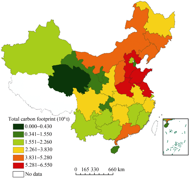
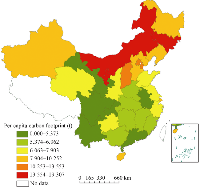
Global warming has been one of the major concerns behind the world’s high-speed economic growth. How to implement the coordinated development of the carbon footprint and the economy will be the core issue of the world’s economic and social development, as well as the heated debate of the research at home and abroad in recent years. Based on the energy consumption, integrated with the “Top-Down” life cycle approach and geographically weighted regression (GWR) model, this paper analyzed the spatial differences and multi-mechanism of carbon footprint in provincial China in 2010. Firstly, this study calculated the amount of carbon footprint of each province using “Top-Down” life cycle approach and found that there were significant differences of carbon footprint and per capita carbon footprint in provincial China. The provinces with higher carbon footprint, mainly located in northern China, have large economic scales; the provinces with higher per capita carbon footprint are mainly distributed in central cities such as Beijing, Shanghai and energy-rich regions and heavy chemical bases. Secondly, with the aid of GIS and spatial analysis model (GWR model), this paper had unfolded that the expansion of economic scale is the main driver of the rapid growth of carbon footprint. The growth of population and urbanization also acted as promoting factors for the increase of the carbon footprint. Energy structure had no considerable promoting effect for the increase of the carbon footprint. Improving energy efficiency is the most important factor to inhibit the growing carbon footprint. Thirdly, developing low-carbon economies and low-carbon industries, as well as advocating low-carbon city construction and improving carbon efficiency would be the primary approaches to inhibit the rapid growth of carbon footprint. Moderately controlling the economic scale and population size would also be required to alleviate carbon footprint. Meanwhile, environmental protection and construction of low-carbon cities would evoke extensive attention in the process of urbanization.
Key words: carbon footprint; spatial differences; multi-mechanism; GWR model; China
WANG Shaojian , FANG Chuanglin , MA Haitao , WANG Yang , QIN Jing . Spatial differences and multi-mechanism of carbon footprint based on GWR model in provincial China[J]. Journal of Geographical Sciences, 2014 , 24(4) : 612 -630 . DOI: 10.1007/s11442-014-1109-z
Figure 1 Spatial distribution of total carbon footprint in provincial China in 2010 |


 <1 is intermediate consumption from unit output of β department to the product of α department.

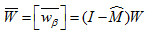
 is the Leontief inverse matrix, donates complete demand of input sector by producing unit final production.
 ):
):

Table 1 Total carbon footprint and per capita carbon footprint in provincial China in 2010 |
| Provincial region | Carbon footprint (108 t) | Per capita carbon footprint (t) | Provincial region | Carbon footprint (108 t) | Per capita carbon footprint (t) | ||
|---|---|---|---|---|---|---|---|
| Beijing | 2.16 | 11.01 | Henan | 5.54 | 5.89 | ||
| Tianjin | 1.46 | 10.28 | Hubei | 3.47 | 6.06 | ||
| Hebei | 6.35 | 8.84 | Hunan | 3.80 | 5.79 | ||
| Shanxi | 4.84 | 13.55 | Guangdong | 5.28 | 5.06 | ||
| Inner Mongolia | 4.77 | 19.31 | Guangxi | 2.62 | 5.69 | ||
| Liaoning | 4.59 | 8.49 | Hainan | 0.78 | 8.99 | ||
| Jilin | 4.38 | 15.95 | Chongqing | 1.55 | 5.37 | ||
| Heilongjiang | 3.25 | 8.48 | Sichuan | 3.46 | 4.30 | ||
| Shanghai | 2.36 | 10.25 | Guizhou | 2.56 | 7.37 | ||
| Jiangsu | 5.81 | 7.39 | Yunnan | 2.30 | 5.00 | ||
| Zhejiang | 3.83 | 7.04 | Shaanxi | 2.95 | 7.90 | ||
| Anhui | 3.06 | 5.14 | Gansu | 1.36 | 5.32 | ||
| Fujian | 2.03 | 5.50 | Qinghai | 0.43 | 7.64 | ||
| Jiangxi | 2.57 | 5.77 | Ningxia | 1.03 | 16.35 | ||
| Shandong | 6.55 | 6.84 | Xinjiang | 2.04 | 9.35 |
Figure 2 Spatial distribution of per capita carbon footprint in provincial China in 2010 |
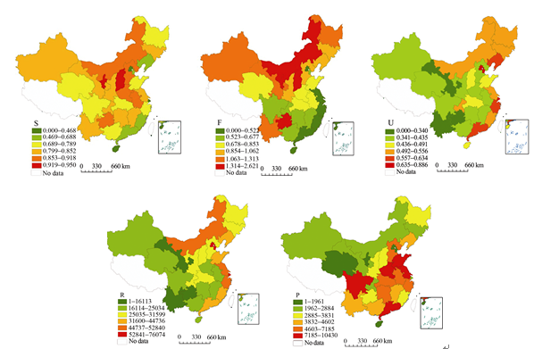
Figure 3 The spatial distribution of five potential determinants in 2010 Notes: energy structure (dominant energy share of total energy consumption), energy efficiency (per unit GDP energy consumption, t/104 yuan), urbanization (urban population/total population), economy factor (per capita GDP, yuan) and population factor (population size, 104 persons) |
Table 2 Descriptive statistics of five factors in 2010 |
| Sstructure (%) | Fefficiency (t/104 yuan) | Uurbanization (%) | Reconomy (104 yuan) | Ppopulation (104 persons) | |
|---|---|---|---|---|---|
| Minimum | 43.48 | 0.29 | 29.9 | 13119.00 | 562.67 |
| Mean | 77.57 | 0.95 | 49.82 | 33964.10 | 4432.58 |
| Maximum | 95.03 | 2.62 | 88.6 | 76074.00 | 10430.31 |
| Standard deviation | 14.75 | 0.57 | 14.29 | 17343.43 | 2707.25 |
Note: Sstructure: energy structure; Fefficiency: energy efficiency; Uurbanization: urbanization level; Reconomy: economic factor; Ppopulation: population factor |
Table 3 Global regression analyses (OLS model) in 2010 |
| OLS model | ||||
|---|---|---|---|---|
| Coefficient | Standard error | t/z-value | Pr(>|t|) | |
| CONSTANT | 0.04598533 | 0.07577884 | -0.606836 | 0.5490287 |
| Sstructure | 0.1226138 | 0.2005283 | -0.6114537 | 0.1460138 |
| Fefficiency | -0.4224572 | 0.1843807 | 2.29122313 | 0.0299797 |
| Uurbanization | 0.0091527 | 0.1504661 | -0.0608201 | 0.0519423 |
| Reconomy | 0.8650346 | 0.0990884 | 2.67472845 | 0.0125450 |
| Ppopulation | 0.4778324 | 0.1223842 | 7.17277265 | 0.0000001 |
| Adjusted R-squared: 0.775289, F-statistic: 23.081 on 2 and 27DF, p-value: 5.67195e-009 | ||||
Note: Sstructure: energy structure; Fefficiency: energy efficiency; Uurbanization: urbanization level; Reconomy: economic factor; Ppopulation: population factor |
Table 4 Global regression analyses (spatial error model) in 2010 |
| Spatial error model | ||||
|---|---|---|---|---|
| Coefficient | Standard error | t/z-value | Pr(>|t|) | |
| CONSTANT | 0.0153703 | 0.0589723 | -0.2606363 | 0.1943731 |
| Sstructure | 0.0038843 | 0.1456612 | 0.02666697 | 0.0787253 |
| Fefficiency | -0.2229032 | 0.1366329 | 1.63140212 | 0.0028055 |
| Uurbanization | 0.0069441 | 0.1119279 | 0.06204101 | 0.1505300 |
| Reconomy | 0.8142238 | 0.0931959 | 1.22563354 | 0.0000000 |
| Ppopulation | 0.4292908 | 0.0918455 | 9.02919169 | 0.0000001 |
| Lambda: 0.787422 LR test value: 8.502896, p-value: 0.0035458, Log likelihood: 27.077155 for error model, AIC: 67.543 (AIC for OLS: 79.231), Robust Lagrange Multiplier test: 2.5314, on 1 DF, p-value: 0.0367 | ||||
Note: Sstructure: energy structure; Fefficiency: energy efficiency; Uurbanization: urbanization level; Reconomy: economic factor; Ppopulation: population factor |
Table 5 Global regression analyses (spatial lag model) in 2010 |
| Spatial lag model | ||||
|---|---|---|---|---|
| Coefficient | Standard error | t/z-value | Pr(>|t|) | |
| CONSTANT | 0.06978879 | 0.0646215 | -1.079962 | 0.2801591 |
| Sstructure | 0.2301915 | 0.1820049 | -1.264755 | 0.2059594 |
| Fefficiency | -0.4195918 | 0.1568021 | 2.675932 | 0.0074523 |
| Uurbanization | 0.0692413 | 0.1309372 | 0.528814 | 0.0969344 |
| Reconomy | 0.8338999 | 0.0913506 | 1.465779 | 0.0000086 |
| Ppopulation | 0.5362292 | 0.1035332 | 8.076922 | 0.0000000 |
| Rho: 0.287546 LR test value: 4.866677, p-value: 0.0273802, Log likelihood: 25.259 for lag model, AIC: 56.5181 (AIC for OLS: 79.231) Robust Lagrange multiplier test:24.328, on 1 DF, p-value: 0.000002354 | ||||
Note: Sstructure: energy structure; Fefficiency: energy efficiency; Uurbanization: urbanization level; Reconomy: economic factor; Ppopulation: population factor |
Table 6 Summary of univariate GWR models for different factors in 2010 |
| Factors | R2 | Significantly related provinces | ||
|---|---|---|---|---|
| p<0.05 (%) | + (%) | - (%) | ||
| Sstructure | 0.62 | 62.4 | 51.2 | 7.6 |
| Fefficiency | 0.67 | 67.5 | 46.8 | 17.2 |
| Uurbanization | 0.56 | 57.7 | 55.6 | 5.9 |
| Recomomy | 0.78 | 77.3 | 75.6 | 4.7 |
| Ppopulation | 0.82 | 89.7 | 88.4 | 2.5 |
Note: Sstructure: energy structure; Fefficiency: energy efficiency; Uurbanization: urbanization level; Reconomy: economic factor; Ppopulation: population factor |
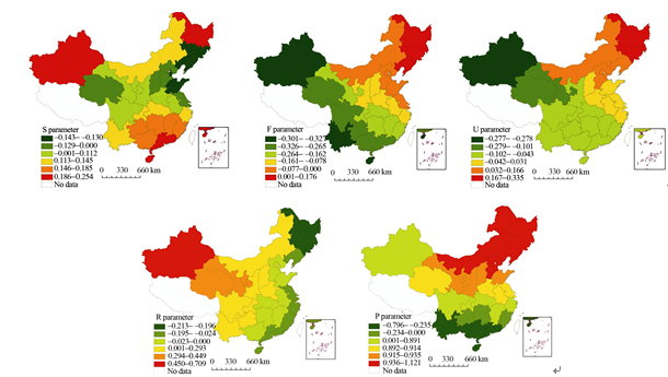
Figure 4 The spatial distribution on the local relationship between carbon footprint and five factors at provincial level in 2010 |
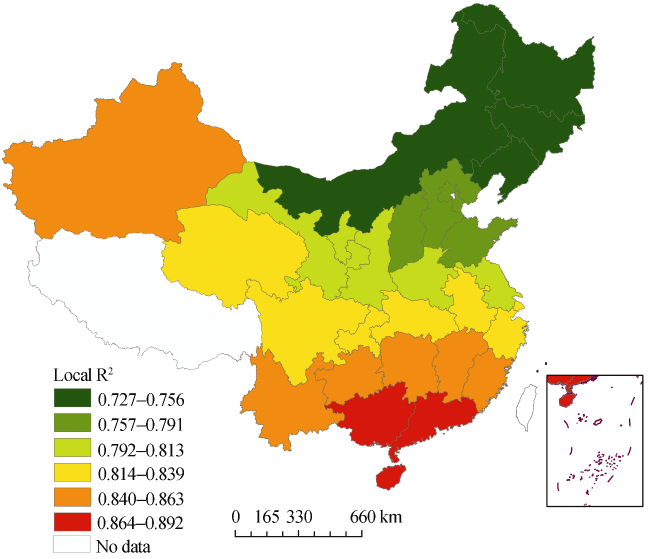
Figure 5 Local R2 derived from mixed GWR model in 2010 |
Table 7 Summary of mixed GWR models for different variables in 2010 |
| The mixed GWR model | ||||
|---|---|---|---|---|
| Coefficient | Standard error | t/z-value | Pr(>|t|) | |
| CONSTANT | 0.0956437 | 0.0446845 | 1.255213 | 0.214675 |
| Sstructure | 0.2541348 | 0.0820820 | -1.112547 | 0.064572 |
| Fefficiency | -0.6278633 | 0.2568357 | 2.364672 | 0.036743 |
| Uurbanization | 0.1859435 | 0.1409965 | 0.867456 | 0.043675 |
| Recomomy | 0.5726534 | 0.0613432 | 0.472894 | 0.002672 |
| Ppopulation | 0.7435687 | 0.0035566 | 2.047683 | 0.000000 |
Note: Sstructure: energy structure; Fefficiency: energy efficiency; Uurbanization: urbanization level; Reconomy: economic factor; Ppopulation: population factor |
Table 8 Comparison of results with other authors |
| Author | Carbon footprint (109 tons) | Year | Reference |
|---|---|---|---|
| Wei Baoren | 1.282 | 2005 | Wei, 2007 |
| Liu Qiang | 1.51 | 2005 | Liu et al., 2008 |
| Xu Guangyue | 1.66 | 2006 | Xu, 2010 |
| Zhao Rongqin | 1.647 | 2007 | Zhao et al., 2011 |
| Shi Minjun | 6.01 | 2007 | Shi et al., 2012 |
| Chuai Xiaowei | 2.05 | 2008 | Chuai et al., 2012 |
| This paper | 9.72 | 2010 |
The authors have declared that no competing interests exist.
| 1 |
|
| 2 |
|
| 3 |
|
| 4 |
|
| 5 |
|
| 6 |
|
| 7 |
|
| 8 |
|
| 9 |
|
| 10 |
|
| 11 |
|
| 12 |
|
| 13 |
|
| 14 |
|
| 15 |
|
| 16 |
IPCC, 2008. Summary for Policymakers of Climate Change 2007: The Physical Science Basis. Contribution of Working Group I to the Fourth Assessment Report of the Intergovernmental Panel on Climate Change. Cambridge: Cambridge University Press.
|
| 17 |
|
| 18 |
|
| 19 |
|
| 20 |
|
| 21 |
|
| 22 |
|
| 23 |
|
| 24 |
|
| 25 |
|
| 26 |
|
| 27 |
|
| 28 |
|
| 29 |
|
| 30 |
|
| 31 |
|
| 32 |
|
| 33 |
|
| 34 |
|
| 35 |
|
| 36 |
|
| 37 |
|
| 38 |
|
| 39 |
|
| 40 |
|
| 41 |
|
| 42 |
|
| 43 |
|
| 44 |
|
| 45 |
|
| 46 |
|
| 47 |
|
| 48 |
|
| 49 |
|
| 50 |
|
| 51 |
|
| 52 |
|
| 53 |
|
| 54 |
|
/
| 〈 |
|
〉 |