Mapping the hotspots and coldspots of ecosystem services in conservation priority setting
Note: When input features are spatially scattered (see
|
Mapping the hotspots and coldspots of ecosystem services in conservation priority setting |
| Yingjie LI, Liwei ZHANG, Junping YAN, Pengtao WANG, Ningke HU, Wei CHENG, Bojie FU |
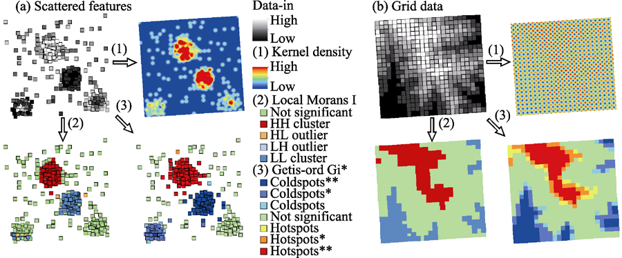
| Figure 7 Comparison of three hotspot analysis methods: KDE (1), Local Moran’s I (2), Getis-Ord Gi* statistics (3) Note: When input features are spatially scattered (see |
|
|